Defining the Stellar Spectrum
In this notebook we provide some examples showing how archNEMESIS can be used to define the stellar spectrum for an atmospheric retrieval.
The main input file for the standard version of NEMESIS is the .sol file, which just includes one line with the name of the file where the solar spectrum is stored. Note this file must be defined in a specific format and it is expected to be stored in Data/stellar/.
On the other hand, in archNEMESIS the information about the solar spectrum is directly written into the input HDF5 file (rather than just using the HDF5 as a pointer to another file).
While the retrievals from archNEMESIS will typically use the input HDF5 file, we also include some built-in methods in the Stellar class to read/write the .sol file and use archNEMESIS as a post or pre-processing tool for standard NEMESIS retrievals.
[1]:
import archnemesis as ans
import matplotlib.pyplot as plt
import numpy as np
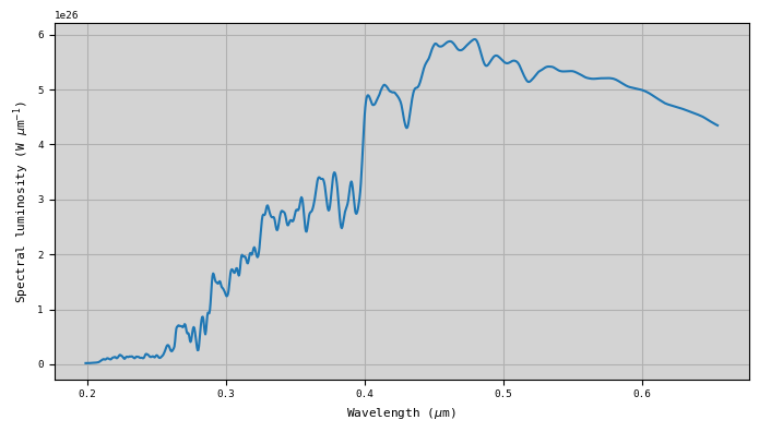
1. Reading the stellar spectrum from the input file
Reading the stellar spectrum from the .sol file
In this example we show how we can use the Stellar class to read the information about the solar spectrum. Here, we are going to create an example .sol file pointing at one of the stellar spectra stored in /Data/stellar/, and we are going to read the file with the Stellar class. Note that the actual file where the stellar spectrum is stored must have a defined format as specified by NEMESIS.
[2]:
#Writing arbitrary .sol file
###############################################################
f = open('example.sol','w')
f.write('houghtonsolar_corr_wl.dat')   #Name of the file containing the information about the solar spectrum
f.close()

#Initialising stellar class and reading .sol file
###############################################################

Stellar = ans.Stellar_0()
Stellar.read_sol('example')

#Making summary plot
###############################################################

fig,ax1 = plt.subplots(1,1,figsize=(7,4))
ax1.plot(Stellar.WAVE,Stellar.SOLSPEC)
ax1.grid()
if Stellar.ISPACE==0:
    ax1.set_xlabel('Wavenumber (cm$^{-1}$)')
    ax1.set_ylabel('Spectral luminosity (W (cm$^{-1}$)$^{-1}$)')
elif Stellar.ISPACE==1:
    ax1.set_xlabel('Wavelength ($\mu$m)')
    ax1.set_ylabel('Spectral luminosity (W $\mu$m$^{-1}$)')
ax1.set_facecolor('lightgray')
plt.tight_layout()
<>:23: SyntaxWarning: invalid escape sequence '\m'
<>:24: SyntaxWarning: invalid escape sequence '\m'
<>:23: SyntaxWarning: invalid escape sequence '\m'
<>:24: SyntaxWarning: invalid escape sequence '\m'
/tmp/ipykernel_2427458/3186311221.py:23: SyntaxWarning: invalid escape sequence '\m'
  ax1.set_xlabel('Wavelength ($\mu$m)')
/tmp/ipykernel_2427458/3186311221.py:24: SyntaxWarning: invalid escape sequence '\m'
  ax1.set_ylabel('Spectral luminosity (W $\mu$m$^{-1}$)')
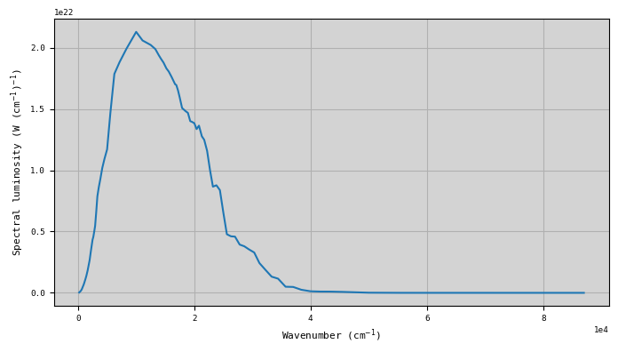
Reading the stellar spectrum from the HDF5 file
In the case that we are reading the information from the HDF5 file, the information about the stellar spectrum is directly stored in this file. Most of the information in the HDF5 file is indeed the information stored in the file under /Data/stellar/. However, in the HDF5 file we also store the information about the planet-star distance.
[3]:
#Initialising class and reading HDF5 file
###################################################

Stellar = ans.Stellar_0()
Stellar.read_hdf5('example')

#Making summary plot
###################################################

fig,ax1 = plt.subplots(1,1,figsize=(7,4))
ax1.plot(Stellar.WAVE,Stellar.SOLSPEC)
ax1.grid()
if Stellar.ISPACE==0:
    ax1.set_xlabel('Wavenumber (cm$^{-1}$)')
    ax1.set_ylabel('Spectral luminosity (W (cm$^{-1}$)$^{-1}$)')
elif Stellar.ISPACE==1:
    ax1.set_xlabel('Wavelength ($\mu$m)')
    ax1.set_ylabel('Spectral luminosity (W $\mu$m$^{-1}$)')
ax1.set_facecolor('lightgray')
plt.tight_layout()
<>:17: SyntaxWarning: invalid escape sequence '\m'
<>:18: SyntaxWarning: invalid escape sequence '\m'
<>:17: SyntaxWarning: invalid escape sequence '\m'
<>:18: SyntaxWarning: invalid escape sequence '\m'
/tmp/ipykernel_2427458/1869230734.py:17: SyntaxWarning: invalid escape sequence '\m'
  ax1.set_xlabel('Wavelength ($\mu$m)')
/tmp/ipykernel_2427458/1869230734.py:18: SyntaxWarning: invalid escape sequence '\m'
  ax1.set_ylabel('Spectral luminosity (W $\mu$m$^{-1}$)')
2. Writing the solar spectrum with the format of the input files
We can also use the Stellar class to write the information about our specific stellar spectrum into the input files requires by NEMESIS and archNEMESIS. In this section, we know how this is performed for each of the two cases.
Creating a new stellar spectrum file
In NEMESIS, the .sol file just points to another file under Data/stellar/ with the information about the stellar spectrum. There are several files stored in this repository, but we may want to create our own for our specific case. In particular, the information we need to know include in the file is:
ISPACE: Units of the stellar spectrum in wavenumber (cm\(^{-1}\); ISPACE=0) or in wavelength (\(\mu\)m; ISPACE=1).
RADIUS: Radius of the star (km)
WAVE: Wavelength at which the solar spectrum is defined.
SOLSPEC: Stellar luminosity (W (cm\(^{-1})^{-1}\) or W \(\mu\)m).
[4]:
#Initialising Stellar class
Stellar = ans.Stellar_0()

#Reading the .sol file
#Here we are reading the information from the .sol file but we may be getting it from other sources
Stellar.read_sol('solspec_wl')

#Writing the new stellar file
Stellar.write_solar_file('example_solar_file.txt')
Writing the archNEMESIS HDF5 file
In archNEMESIS, we directly include the information about the stellar spectrum in the input HDF5 file, but the information we require is indeed the same. Note that the Planet-Star distance is another parameter in the Stellar class, and this information also needs to be defined to write the HDF5 file apart from the stellar spectrum itself.
[5]:
#Initialising Stellar class
Stellar = ans.Stellar_0()

#Reading the .sol file
#Here we are reading the information from the .sol file but we may be getting it from other sources
Stellar.read_sol('solspec_wl')

#Defining the planet-star distance
Stellar.DIST = 1.0   #Earth distance

#Writing the HDF5 file
Stellar.write_hdf5('example_hdf5')
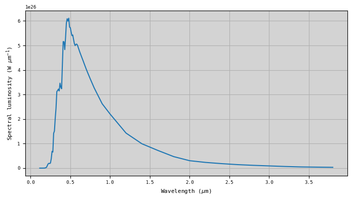
We may define the stellar spectrum ourselves, but we may also want to use the information in the Data/stellar/ files used by NEMESIS. In this case, we just need use the optional input solfile in the Stellar.write_hdf5() method.
Here, we are going to write the information in the solspec_tsis1-sim.dat file under Data/stellar/.
[6]:
#Initialising Stellar class
Stellar = ans.Stellar_0()

#Defining the planet-star distance
Stellar.DIST = 1.0   #Earth distance

#Writing the information into HDF5 file
Stellar.write_hdf5('example_hdf5',solfile='solspec_tsis1-sim.dat')

#Reading the HDF5 file
Stellar.read_hdf5('example_hdf5')

#Making plot of the spectrum
fig,ax1 = plt.subplots(1,1,figsize=(7,4))
ax1.plot(Stellar.WAVE,Stellar.SOLSPEC)
ax1.grid()
if Stellar.ISPACE==0:
    ax1.set_xlabel('Wavenumber (cm$^{-1}$)')
    ax1.set_ylabel('Spectral luminosity (W (cm$^{-1}$)$^{-1}$)')
elif Stellar.ISPACE==1:
    ax1.set_xlabel('Wavelength ($\mu$m)')
    ax1.set_ylabel('Spectral luminosity (W $\mu$m$^{-1}$)')
ax1.set_facecolor('lightgray')
plt.tight_layout()
<>:21: SyntaxWarning: invalid escape sequence '\m'
<>:22: SyntaxWarning: invalid escape sequence '\m'
<>:21: SyntaxWarning: invalid escape sequence '\m'
<>:22: SyntaxWarning: invalid escape sequence '\m'
/tmp/ipykernel_2427458/1745539258.py:21: SyntaxWarning: invalid escape sequence '\m'
  ax1.set_xlabel('Wavelength ($\mu$m)')
/tmp/ipykernel_2427458/1745539258.py:22: SyntaxWarning: invalid escape sequence '\m'
  ax1.set_ylabel('Spectral luminosity (W $\mu$m$^{-1}$)')
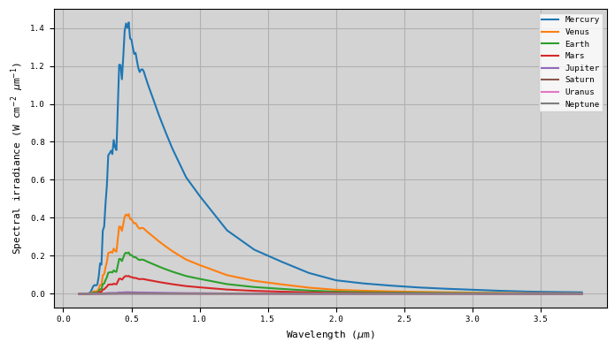
3. Calculating the solar irradiance at a given distance
Once the stellar spectrum has been read, the stellar flux or irradiance at a given distance to the star can be easily calculated following
\begin{equation} F(\lambda,d) = \dfrac{P(\lambda)}{4 \pi d^2}, \end{equation}
where \(P(\lambda)\) is the stellar spectral luminosity and \(d\) is the distance from the planet to the star. This calculation can be performed in the Stellar class using the method calc_solar_flux(), and the information about this parameter is stored under Stellar.SOLFLUX.
[7]:
#Initialising Stellar class
Stellar = ans.Stellar_0()

#Reading the .sol file
Stellar.read_sol('solspec_wl')

#Defining a range of planet-Sun distances
dist = [0.39,0.72,1.,1.52,5.2,9.54,19.22,30.06]
labels = ['Mercury','Venus','Earth','Mars','Jupiter','Saturn','Uranus','Neptune']

#Making a plot with the flux at the different planets
fig,ax1 = plt.subplots(1,1,figsize=(7,4))

for i in range(8):

    #Defining the distance to star
    Stellar.DIST = dist[i]   #Planet-Star distance in Astronomical Units

    #Calculating the flux
    Stellar.calc_solar_flux()

    ax1.plot(Stellar.WAVE,Stellar.SOLFLUX,label=labels[i])

ax1.grid()
ax1.legend()
#ax1.set_yscale('log')
if Stellar.ISPACE==0:
    ax1.set_xlabel('Wavenumber (cm$^{-1}$)')
    ax1.set_ylabel('Spectral irradiance (W cm$^{-2}$ (cm$^{-1}$)$^{-1}$)')
elif Stellar.ISPACE==1:
    ax1.set_xlabel('Wavelength ($\mu$m)')
    ax1.set_ylabel('Spectral irradiance (W cm$^{-2}$ $\mu$m$^{-1}$)')
ax1.set_facecolor('lightgray')
plt.tight_layout()
<>:31: SyntaxWarning: invalid escape sequence '\m'
<>:32: SyntaxWarning: invalid escape sequence '\m'
<>:31: SyntaxWarning: invalid escape sequence '\m'
<>:32: SyntaxWarning: invalid escape sequence '\m'
/tmp/ipykernel_2427458/674966289.py:31: SyntaxWarning: invalid escape sequence '\m'
  ax1.set_xlabel('Wavelength ($\mu$m)')
/tmp/ipykernel_2427458/674966289.py:32: SyntaxWarning: invalid escape sequence '\m'
  ax1.set_ylabel('Spectral irradiance (W cm$^{-2}$ $\mu$m$^{-1}$)')
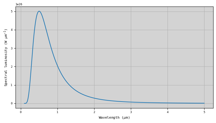
4. Modelling the stellar spectrum as a blackbody
In some cases, we may not have enough information about the stellar spectrum, but we may assume it follows the blackbody emission at a given temperature. In that case, we can calculate the star luminosity as
\begin{equation} L = 4\pi^2 \cdot R_{*}^2 \cdot B(T_*). \end{equation}
We can easily perform this calculation using the functionality of the Stellar class.
[8]:
#Initialising class
Stellar = ans.Stellar_0()

Stellar.RADIUS = 6.957e5  #Radius of the star (km)
Stellar.ISPACE = 1        #Wavelength (um)
Stellar.NWAVE = 1001
Stellar.WAVE = np.linspace(0.1,5.,Stellar.NWAVE)

#Calculating the stellar luminosity from the blackbody
T_star = 5772.
Stellar.calc_luminosity_blackbody(T_star)

#Making summary plot
###############################################################

fig,ax1 = plt.subplots(1,1,figsize=(7,4))
ax1.plot(Stellar.WAVE,Stellar.SOLSPEC)
ax1.grid()
if Stellar.ISPACE==0:
    ax1.set_xlabel('Wavenumber (cm$^{-1}$)')
    ax1.set_ylabel('Spectral luminosity (W (cm$^{-1}$)$^{-1}$)')
elif Stellar.ISPACE==1:
    ax1.set_xlabel('Wavelength ($\mu$m)')
    ax1.set_ylabel('Spectral luminosity (W $\mu$m$^{-1}$)')
ax1.set_facecolor('lightgray')
plt.tight_layout()
<>:23: SyntaxWarning: invalid escape sequence '\m'
<>:24: SyntaxWarning: invalid escape sequence '\m'
<>:23: SyntaxWarning: invalid escape sequence '\m'
<>:24: SyntaxWarning: invalid escape sequence '\m'
/tmp/ipykernel_2427458/3758227508.py:23: SyntaxWarning: invalid escape sequence '\m'
  ax1.set_xlabel('Wavelength ($\mu$m)')
/tmp/ipykernel_2427458/3758227508.py:24: SyntaxWarning: invalid escape sequence '\m'
  ax1.set_ylabel('Spectral luminosity (W $\mu$m$^{-1}$)')