Defining the layering of the atmosphere
In this notebook, we want to have a closer look to the Layer class of archNEMESIS. In a forward model or retrieval, we usually define the input atmospheric profiles (e.g., altitude, pressure, temperature, volume mixing ratio, dust abundance, etc.). However, for the radiative transfer calculations we need to define a finite number of layers, with a specified width, pressure and temperature. The Layer class is specifically designed to make this transformation from the initial vertical profiles in our Atmosphere, to the layers at which the radiative transfer calculations are defined.
Apart from the reference atmospheric profiles, the main inputs we need to define how to split our atmosphere into layers and calculate their properties are:
RADIUS: Reference planetary radius where H=0. Usually at surface for terrestrial planets, or at 1 bar pressure level for gas giants.
NLAY: Defines the number of layers we want to include in the atmosphere
LAYHT: Height of the base of the lowest layer (m). Default is 0.
LAYANG: Angle from the zenith at which to split up the layers. Default is 0.
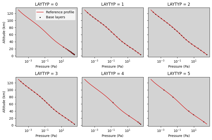
LAYTYP: Integer specifying how to split up the layers. In NEMESIS, it can take up to six values:
LAYTYP=0: Layers are split by equal changes in pressure.
LAYTYP=1: Layers are split by equal changes in log pressure.
LAYTYP=2: Layers are split by equal changes in height.
LAYTYP=3: Layers are split by equal changes in path length at LAYANG.
LAYTYP=4: Base pressure of the layers is explicitly specified by P_base.
LAYTYP=5: Base altitude of the layers is explicitly specified by H_base.
LAYINT: Integer specifying how the effective properties of the layer (i.e., temperature and pressure) should be calculated.
LAYINT=0: Layer properties are taken at the middle of the layer.
LAYINT=1: Layer properties calculated by performing a weighted average on the layer with the absorber amounts. This option is generally recommended, but LAYINT=0 might be useful for comparisons.
Once the inputs of the Layer class have been defined, we can simply use the main function of the Layer class, Layer.calc_layering(), to split the atmosphere into layers and calculate their effective properties. The inputs to this function are the internal parameters of the class, and the reference atmospheric profiles (typically taken from the Atmosphere class).
[1]:
import archnemesis as ans
import matplotlib.pyplot as plt
import numpy as np
1. Splitting the atmosphere into layers
In this notebook we are going to split the atmosphere into different layers using the several methods that are supported by NEMESIS. To do so, we are going to take some reference profiles from the Martian atmosphere and are going to test the different values of LAYTYP. The function to split the atmosphere into layers is called Layer.layer_split(), but we could also perform these calculations with the more complete Layer.calc_layering() function, which does these calculations and also calcualtes the effective properties of the layers.
[2]:
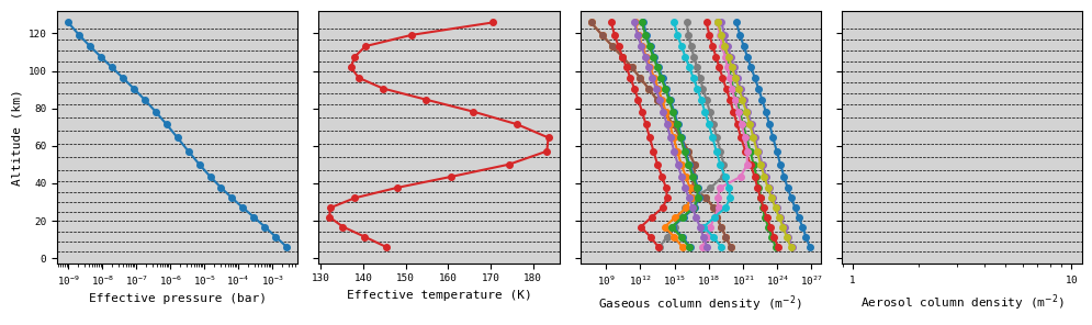
#Reading reference atmospheric profiles
################################################

Atmosphere = ans.Atmosphere_0()
Atmosphere.read_hdf5('mars')

#Defining the inputs for the Layer class
#################################################

Layer = ans.Layer_0()

Layer.RADIUS = Atmosphere.RADIUS #Radius of the planet (m)
Layer.LAYANG = 0.0   #Angle at which to split the layers (typically it is zero)
Layer.NLAY = 21      #Number of atmospheric layers
Layer.LAYHT = 0.0


#Calculating the layer base heights and pressures for the different methods
##################################################################################

fig,ax = plt.subplots(2,3,figsize=(9,6),sharey=True)

#Equal changes in pressure
Layer.LAYTYP = 0
Layer.layer_split(H=Atmosphere.H, P=Atmosphere.P, T=Atmosphere.T, LAYANG=Layer.LAYANG)

ax[0,Layer.LAYTYP].plot(Atmosphere.P,Atmosphere.H/1.0e3,c='tab:red',label='Reference profile')
ax[0,Layer.LAYTYP].scatter(Layer.BASEP,Layer.BASEH/1.0e3,s=5.,c='black',label='Base layers')
ax[0,Layer.LAYTYP].set_xscale('log')
ax[0,Layer.LAYTYP].set_title('LAYTYP = '+str(Layer.LAYTYP))
ax[0,Layer.LAYTYP].set_facecolor('lightgray')
ax[0,Layer.LAYTYP].set_xlabel('Pressure (Pa)')
ax[0,Layer.LAYTYP].legend()


#Equal changes in log pressure
Layer.LAYTYP = 1
Layer.layer_split(H=Atmosphere.H, P=Atmosphere.P, T=Atmosphere.T, LAYANG=Layer.LAYANG)

ax[0,Layer.LAYTYP].plot(Atmosphere.P,Atmosphere.H/1.0e3,c='tab:red')
ax[0,Layer.LAYTYP].scatter(Layer.BASEP,Layer.BASEH/1.0e3,s=5.,c='black')
ax[0,Layer.LAYTYP].set_xscale('log')
ax[0,Layer.LAYTYP].set_title('LAYTYP = '+str(Layer.LAYTYP))
ax[0,Layer.LAYTYP].set_facecolor('lightgray')
ax[0,Layer.LAYTYP].set_xlabel('Pressure (Pa)')

#Equal changes in height
Layer.LAYTYP = 2
Layer.layer_split(H=Atmosphere.H, P=Atmosphere.P, T=Atmosphere.T, LAYANG=Layer.LAYANG)

ax[0,Layer.LAYTYP].plot(Atmosphere.P,Atmosphere.H/1.0e3,c='tab:red')
ax[0,Layer.LAYTYP].scatter(Layer.BASEP,Layer.BASEH/1.0e3,s=5.,c='black')
ax[0,Layer.LAYTYP].set_xscale('log')
ax[0,Layer.LAYTYP].set_title('LAYTYP = '+str(Layer.LAYTYP))
ax[0,Layer.LAYTYP].set_facecolor('lightgray')
ax[0,Layer.LAYTYP].set_xlabel('Pressure (Pa)')


#Equal changes in line-of-sight path intervals
Layer.LAYTYP = 3
Layer.layer_split(H=Atmosphere.H, P=Atmosphere.P, T=Atmosphere.T, LAYANG=Layer.LAYANG)

ax[1,Layer.LAYTYP-3].plot(Atmosphere.P,Atmosphere.H/1.0e3,c='tab:red')
ax[1,Layer.LAYTYP-3].scatter(Layer.BASEP,Layer.BASEH/1.0e3,s=5.,c='black')
ax[1,Layer.LAYTYP-3].set_xscale('log')
ax[1,Layer.LAYTYP-3].set_title('LAYTYP = '+str(Layer.LAYTYP))
ax[1,Layer.LAYTYP-3].set_facecolor('lightgray')
ax[1,Layer.LAYTYP-3].set_xlabel('Pressure (Pa)')

#Specify base pressures
Layer.LAYTYP = 4
Layer.P_base = np.array([369.233, 263.738, 175.8259, 14.660, 0.16523462])

Layer.layer_split(H=Atmosphere.H, P=Atmosphere.P, T=Atmosphere.T, LAYANG=Layer.LAYANG)

ax[1,Layer.LAYTYP-3].plot(Atmosphere.P,Atmosphere.H/1.0e3,c='tab:red')
ax[1,Layer.LAYTYP-3].scatter(Layer.BASEP,Layer.BASEH/1.0e3,s=5.,c='black')
ax[1,Layer.LAYTYP-3].set_xscale('log')
ax[1,Layer.LAYTYP-3].set_title('LAYTYP = '+str(Layer.LAYTYP))
ax[1,Layer.LAYTYP-3].set_facecolor('lightgray')
ax[1,Layer.LAYTYP-3].set_xlabel('Pressure (Pa)')


#Specify base altitudes
Layer.LAYTYP = 5
Layer.H_base = np.array([10.,30.,40.,80.,100.])*1.0e3

Layer.layer_split(H=Atmosphere.H, P=Atmosphere.P, T=Atmosphere.T, LAYANG=Layer.LAYANG)

ax[1,Layer.LAYTYP-3].plot(Atmosphere.P,Atmosphere.H/1.0e3,c='tab:red')
ax[1,Layer.LAYTYP-3].scatter(Layer.BASEP,Layer.BASEH/1.0e3,s=5.,c='black')
ax[1,Layer.LAYTYP-3].set_xscale('log')
ax[1,Layer.LAYTYP-3].set_title('LAYTYP = '+str(Layer.LAYTYP))
ax[1,Layer.LAYTYP-3].set_facecolor('lightgray')
ax[1,Layer.LAYTYP-3].set_xlabel('Pressure (Pa)')

ax[0,0].set_ylabel('Altitude (km)')
ax[1,0].set_ylabel('Altitude (km)')

plt.tight_layout()
WARNING :: layer_split :: Layer_0.py-1450 ::  from layer_split() :: LAYHT < H(0). Resetting LAYHT
WARNING :: layer_split :: Layer_0.py-1450 ::  from layer_split() :: LAYHT < H(0). Resetting LAYHT
WARNING :: layer_split :: Layer_0.py-1450 ::  from layer_split() :: LAYHT < H(0). Resetting LAYHT
WARNING :: layer_split :: Layer_0.py-1450 ::  from layer_split() :: LAYHT < H(0). Resetting LAYHT
WARNING :: layer_split :: Layer_0.py-1450 ::  from layer_split() :: LAYHT < H(0). Resetting LAYHT
WARNING :: layer_split :: Layer_0.py-1450 ::  from layer_split() :: LAYHT < H(0). Resetting LAYHT
2. Calculating the layer effective parameters
Once the atmosphere has been split into layers, we need to compute the effective properties of each layer so that we can perform the radiative transfer calculations.
[3]:
#Splitting the atmosphere into layers and calculating their effective properties
#############################################################################################

Layer.LAYTYP= 1
Layer.NLAY = 21
Layer.calc_layering(H=Atmosphere.H,P=Atmosphere.P,T=Atmosphere.T, ID=Atmosphere.ID,VMR=Atmosphere.VMR, DUST=Atmosphere.DUST, PARAH2=Atmosphere.PARAH2)

#Printing some useful information
#############################################################################################

#Printing some useful information in the screen
Layer.summary_info()

#Making a summary plot
Layer.plot_Layer()
WARNING :: layer_split :: Layer_0.py-1450 ::  from layer_split() :: LAYHT < H(0). Resetting LAYHT
INFO :: summary_info :: Layer_0.py-253 :: Number of layers ::  21
INFO :: summary_info :: Layer_0.py-258 :: Layers calculated by equal changes in log pressure
INFO :: summary_info :: Layer_0.py-271 :: Layer properties calculated through mass weighted averages
INFO :: summary_info :: Layer_0.py-274 :: BASEH(km) ('BASEP(bar)', 'DELH(km)', 'P(bar)', 'T(K)', 'TOTAM(m-2)', 'DUST_TOTAM(m-2)')
--- Logging error ---
Traceback (most recent call last):
  File "/home/dobinsonl/.local/.python/3.13.0/lib/python3.13/logging/__init__.py", line 1150, in emit
    msg = self.format(record)
  File "/home/dobinsonl/.local/.python/3.13.0/lib/python3.13/logging/__init__.py", line 998, in format
    return fmt.format(record)
           ~~~~~~~~~~^^^^^^^^
  File "/home/dobinsonl/.local/.python/3.13.0/lib/python3.13/logging/__init__.py", line 711, in format
    record.message = record.getMessage()
                     ~~~~~~~~~~~~~~~~~^^
  File "/home/dobinsonl/.local/.python/3.13.0/lib/python3.13/logging/__init__.py", line 400, in getMessage
    msg = msg % self.args
          ~~~~^~~~~~~~~~~
TypeError: not all arguments converted during string formatting
Call stack:
  File "<frozen runpy>", line 198, in _run_module_as_main
  File "<frozen runpy>", line 88, in _run_code
  File "/home/dobinsonl/repos/archnemesis-dist/.venv/lib/python3.13/site-packages/ipykernel_launcher.py", line 18, in <module>
    app.launch_new_instance()
  File "/home/dobinsonl/repos/archnemesis-dist/.venv/lib/python3.13/site-packages/traitlets/config/application.py", line 1075, in launch_instance
    app.start()
  File "/home/dobinsonl/repos/archnemesis-dist/.venv/lib/python3.13/site-packages/ipykernel/kernelapp.py", line 739, in start
    self.io_loop.start()
  File "/home/dobinsonl/repos/archnemesis-dist/.venv/lib/python3.13/site-packages/tornado/platform/asyncio.py", line 211, in start
    self.asyncio_loop.run_forever()
  File "/home/dobinsonl/.local/.python/3.13.0/lib/python3.13/asyncio/base_events.py", line 679, in run_forever
    self._run_once()
  File "/home/dobinsonl/.local/.python/3.13.0/lib/python3.13/asyncio/base_events.py", line 2027, in _run_once
    handle._run()
  File "/home/dobinsonl/.local/.python/3.13.0/lib/python3.13/asyncio/events.py", line 89, in _run
    self._context.run(self._callback, *self._args)
  File "/home/dobinsonl/repos/archnemesis-dist/.venv/lib/python3.13/site-packages/ipykernel/kernelbase.py", line 519, in dispatch_queue
    await self.process_one()
  File "/home/dobinsonl/repos/archnemesis-dist/.venv/lib/python3.13/site-packages/ipykernel/kernelbase.py", line 508, in process_one
    await dispatch(*args)
  File "/home/dobinsonl/repos/archnemesis-dist/.venv/lib/python3.13/site-packages/ipykernel/kernelbase.py", line 400, in dispatch_shell
    await result
  File "/home/dobinsonl/repos/archnemesis-dist/.venv/lib/python3.13/site-packages/ipykernel/ipkernel.py", line 368, in execute_request
    await super().execute_request(stream, ident, parent)
  File "/home/dobinsonl/repos/archnemesis-dist/.venv/lib/python3.13/site-packages/ipykernel/kernelbase.py", line 767, in execute_request
    reply_content = await reply_content
  File "/home/dobinsonl/repos/archnemesis-dist/.venv/lib/python3.13/site-packages/ipykernel/ipkernel.py", line 455, in do_execute
    res = shell.run_cell(
  File "/home/dobinsonl/repos/archnemesis-dist/.venv/lib/python3.13/site-packages/ipykernel/zmqshell.py", line 577, in run_cell
    return super().run_cell(*args, **kwargs)
  File "/home/dobinsonl/repos/archnemesis-dist/.venv/lib/python3.13/site-packages/IPython/core/interactiveshell.py", line 3116, in run_cell
    result = self._run_cell(
  File "/home/dobinsonl/repos/archnemesis-dist/.venv/lib/python3.13/site-packages/IPython/core/interactiveshell.py", line 3171, in _run_cell
    result = runner(coro)
  File "/home/dobinsonl/repos/archnemesis-dist/.venv/lib/python3.13/site-packages/IPython/core/async_helpers.py", line 128, in _pseudo_sync_runner
    coro.send(None)
  File "/home/dobinsonl/repos/archnemesis-dist/.venv/lib/python3.13/site-packages/IPython/core/interactiveshell.py", line 3394, in run_cell_async
    has_raised = await self.run_ast_nodes(code_ast.body, cell_name,
  File "/home/dobinsonl/repos/archnemesis-dist/.venv/lib/python3.13/site-packages/IPython/core/interactiveshell.py", line 3639, in run_ast_nodes
    if await self.run_code(code, result, async_=asy):
  File "/home/dobinsonl/repos/archnemesis-dist/.venv/lib/python3.13/site-packages/IPython/core/interactiveshell.py", line 3699, in run_code
    exec(code_obj, self.user_global_ns, self.user_ns)
  File "/tmp/ipykernel_2426591/3540087341.py", line 12, in <module>
    Layer.summary_info()
  File "/home/dobinsonl/repos/archnemesis-dist/archnemesis/Layer_0.py", line 276, in summary_info
    _lgr.info(self.BASEH[i]/1.0e3,self.BASEP[i]/1.0e5,self.DELH[i]/1.0e3,self.PRESS[i]/1.0e5,self.TEMP[i],np.sum(self.AMOUNT[i,:]),np.sum(self.CONT[i,:]))
Message: np.float64(3.424995893212529)
Arguments: (np.float64(0.0036923434448242203), np.float64(5.617526329736962), np.float64(0.0027521430538672534), np.float64(145.48803856834152), np.float64(7.370279835574325e+26), np.float64(0.0))
--- Logging error ---
Traceback (most recent call last):
  File "/home/dobinsonl/.local/.python/3.13.0/lib/python3.13/logging/__init__.py", line 1150, in emit
    msg = self.format(record)
  File "/home/dobinsonl/.local/.python/3.13.0/lib/python3.13/logging/__init__.py", line 998, in format
    return fmt.format(record)
           ~~~~~~~~~~^^^^^^^^
  File "/home/dobinsonl/.local/.python/3.13.0/lib/python3.13/logging/__init__.py", line 711, in format
    record.message = record.getMessage()
                     ~~~~~~~~~~~~~~~~~^^
  File "/home/dobinsonl/.local/.python/3.13.0/lib/python3.13/logging/__init__.py", line 400, in getMessage
    msg = msg % self.args
          ~~~~^~~~~~~~~~~
TypeError: not all arguments converted during string formatting
Call stack:
  File "<frozen runpy>", line 198, in _run_module_as_main
  File "<frozen runpy>", line 88, in _run_code
  File "/home/dobinsonl/repos/archnemesis-dist/.venv/lib/python3.13/site-packages/ipykernel_launcher.py", line 18, in <module>
    app.launch_new_instance()
  File "/home/dobinsonl/repos/archnemesis-dist/.venv/lib/python3.13/site-packages/traitlets/config/application.py", line 1075, in launch_instance
    app.start()
  File "/home/dobinsonl/repos/archnemesis-dist/.venv/lib/python3.13/site-packages/ipykernel/kernelapp.py", line 739, in start
    self.io_loop.start()
  File "/home/dobinsonl/repos/archnemesis-dist/.venv/lib/python3.13/site-packages/tornado/platform/asyncio.py", line 211, in start
    self.asyncio_loop.run_forever()
  File "/home/dobinsonl/.local/.python/3.13.0/lib/python3.13/asyncio/base_events.py", line 679, in run_forever
    self._run_once()
  File "/home/dobinsonl/.local/.python/3.13.0/lib/python3.13/asyncio/base_events.py", line 2027, in _run_once
    handle._run()
  File "/home/dobinsonl/.local/.python/3.13.0/lib/python3.13/asyncio/events.py", line 89, in _run
    self._context.run(self._callback, *self._args)
  File "/home/dobinsonl/repos/archnemesis-dist/.venv/lib/python3.13/site-packages/ipykernel/kernelbase.py", line 519, in dispatch_queue
    await self.process_one()
  File "/home/dobinsonl/repos/archnemesis-dist/.venv/lib/python3.13/site-packages/ipykernel/kernelbase.py", line 508, in process_one
    await dispatch(*args)
  File "/home/dobinsonl/repos/archnemesis-dist/.venv/lib/python3.13/site-packages/ipykernel/kernelbase.py", line 400, in dispatch_shell
    await result
  File "/home/dobinsonl/repos/archnemesis-dist/.venv/lib/python3.13/site-packages/ipykernel/ipkernel.py", line 368, in execute_request
    await super().execute_request(stream, ident, parent)
  File "/home/dobinsonl/repos/archnemesis-dist/.venv/lib/python3.13/site-packages/ipykernel/kernelbase.py", line 767, in execute_request
    reply_content = await reply_content
  File "/home/dobinsonl/repos/archnemesis-dist/.venv/lib/python3.13/site-packages/ipykernel/ipkernel.py", line 455, in do_execute
    res = shell.run_cell(
  File "/home/dobinsonl/repos/archnemesis-dist/.venv/lib/python3.13/site-packages/ipykernel/zmqshell.py", line 577, in run_cell
    return super().run_cell(*args, **kwargs)
  File "/home/dobinsonl/repos/archnemesis-dist/.venv/lib/python3.13/site-packages/IPython/core/interactiveshell.py", line 3116, in run_cell
    result = self._run_cell(
  File "/home/dobinsonl/repos/archnemesis-dist/.venv/lib/python3.13/site-packages/IPython/core/interactiveshell.py", line 3171, in _run_cell
    result = runner(coro)
  File "/home/dobinsonl/repos/archnemesis-dist/.venv/lib/python3.13/site-packages/IPython/core/async_helpers.py", line 128, in _pseudo_sync_runner
    coro.send(None)
  File "/home/dobinsonl/repos/archnemesis-dist/.venv/lib/python3.13/site-packages/IPython/core/interactiveshell.py", line 3394, in run_cell_async
    has_raised = await self.run_ast_nodes(code_ast.body, cell_name,
  File "/home/dobinsonl/repos/archnemesis-dist/.venv/lib/python3.13/site-packages/IPython/core/interactiveshell.py", line 3639, in run_ast_nodes
    if await self.run_code(code, result, async_=asy):
  File "/home/dobinsonl/repos/archnemesis-dist/.venv/lib/python3.13/site-packages/IPython/core/interactiveshell.py", line 3699, in run_code
    exec(code_obj, self.user_global_ns, self.user_ns)
  File "/tmp/ipykernel_2426591/3540087341.py", line 12, in <module>
    Layer.summary_info()
  File "/home/dobinsonl/repos/archnemesis-dist/archnemesis/Layer_0.py", line 276, in summary_info
    _lgr.info(self.BASEH[i]/1.0e3,self.BASEP[i]/1.0e5,self.DELH[i]/1.0e3,self.PRESS[i]/1.0e5,self.TEMP[i],np.sum(self.AMOUNT[i,:]),np.sum(self.CONT[i,:]))
Message: np.float64(9.04252222294949)
Arguments: (np.float64(0.0017608174868068514), np.float64(5.314357101379221), np.float64(0.0012946058163291346), np.float64(140.38816201279914), np.float64(3.406107491795587e+26), np.float64(0.0))
--- Logging error ---
Traceback (most recent call last):
  File "/home/dobinsonl/.local/.python/3.13.0/lib/python3.13/logging/__init__.py", line 1150, in emit
    msg = self.format(record)
  File "/home/dobinsonl/.local/.python/3.13.0/lib/python3.13/logging/__init__.py", line 998, in format
    return fmt.format(record)
           ~~~~~~~~~~^^^^^^^^
  File "/home/dobinsonl/.local/.python/3.13.0/lib/python3.13/logging/__init__.py", line 711, in format
    record.message = record.getMessage()
                     ~~~~~~~~~~~~~~~~~^^
  File "/home/dobinsonl/.local/.python/3.13.0/lib/python3.13/logging/__init__.py", line 400, in getMessage
    msg = msg % self.args
          ~~~~^~~~~~~~~~~
TypeError: not all arguments converted during string formatting
Call stack:
  File "<frozen runpy>", line 198, in _run_module_as_main
  File "<frozen runpy>", line 88, in _run_code
  File "/home/dobinsonl/repos/archnemesis-dist/.venv/lib/python3.13/site-packages/ipykernel_launcher.py", line 18, in <module>
    app.launch_new_instance()
  File "/home/dobinsonl/repos/archnemesis-dist/.venv/lib/python3.13/site-packages/traitlets/config/application.py", line 1075, in launch_instance
    app.start()
  File "/home/dobinsonl/repos/archnemesis-dist/.venv/lib/python3.13/site-packages/ipykernel/kernelapp.py", line 739, in start
    self.io_loop.start()
  File "/home/dobinsonl/repos/archnemesis-dist/.venv/lib/python3.13/site-packages/tornado/platform/asyncio.py", line 211, in start
    self.asyncio_loop.run_forever()
  File "/home/dobinsonl/.local/.python/3.13.0/lib/python3.13/asyncio/base_events.py", line 679, in run_forever
    self._run_once()
  File "/home/dobinsonl/.local/.python/3.13.0/lib/python3.13/asyncio/base_events.py", line 2027, in _run_once
    handle._run()
  File "/home/dobinsonl/.local/.python/3.13.0/lib/python3.13/asyncio/events.py", line 89, in _run
    self._context.run(self._callback, *self._args)
  File "/home/dobinsonl/repos/archnemesis-dist/.venv/lib/python3.13/site-packages/ipykernel/kernelbase.py", line 519, in dispatch_queue
    await self.process_one()
  File "/home/dobinsonl/repos/archnemesis-dist/.venv/lib/python3.13/site-packages/ipykernel/kernelbase.py", line 508, in process_one
    await dispatch(*args)
  File "/home/dobinsonl/repos/archnemesis-dist/.venv/lib/python3.13/site-packages/ipykernel/kernelbase.py", line 400, in dispatch_shell
    await result
  File "/home/dobinsonl/repos/archnemesis-dist/.venv/lib/python3.13/site-packages/ipykernel/ipkernel.py", line 368, in execute_request
    await super().execute_request(stream, ident, parent)
  File "/home/dobinsonl/repos/archnemesis-dist/.venv/lib/python3.13/site-packages/ipykernel/kernelbase.py", line 767, in execute_request
    reply_content = await reply_content
  File "/home/dobinsonl/repos/archnemesis-dist/.venv/lib/python3.13/site-packages/ipykernel/ipkernel.py", line 455, in do_execute
    res = shell.run_cell(
  File "/home/dobinsonl/repos/archnemesis-dist/.venv/lib/python3.13/site-packages/ipykernel/zmqshell.py", line 577, in run_cell
    return super().run_cell(*args, **kwargs)
  File "/home/dobinsonl/repos/archnemesis-dist/.venv/lib/python3.13/site-packages/IPython/core/interactiveshell.py", line 3116, in run_cell
    result = self._run_cell(
  File "/home/dobinsonl/repos/archnemesis-dist/.venv/lib/python3.13/site-packages/IPython/core/interactiveshell.py", line 3171, in _run_cell
    result = runner(coro)
  File "/home/dobinsonl/repos/archnemesis-dist/.venv/lib/python3.13/site-packages/IPython/core/async_helpers.py", line 128, in _pseudo_sync_runner
    coro.send(None)
  File "/home/dobinsonl/repos/archnemesis-dist/.venv/lib/python3.13/site-packages/IPython/core/interactiveshell.py", line 3394, in run_cell_async
    has_raised = await self.run_ast_nodes(code_ast.body, cell_name,
  File "/home/dobinsonl/repos/archnemesis-dist/.venv/lib/python3.13/site-packages/IPython/core/interactiveshell.py", line 3639, in run_ast_nodes
    if await self.run_code(code, result, async_=asy):
  File "/home/dobinsonl/repos/archnemesis-dist/.venv/lib/python3.13/site-packages/IPython/core/interactiveshell.py", line 3699, in run_code
    exec(code_obj, self.user_global_ns, self.user_ns)
  File "/tmp/ipykernel_2426591/3540087341.py", line 12, in <module>
    Layer.summary_info()
  File "/home/dobinsonl/repos/archnemesis-dist/archnemesis/Layer_0.py", line 276, in summary_info
    _lgr.info(self.BASEH[i]/1.0e3,self.BASEP[i]/1.0e5,self.DELH[i]/1.0e3,self.PRESS[i]/1.0e5,self.TEMP[i],np.sum(self.AMOUNT[i,:]),np.sum(self.CONT[i,:]))
Message: np.float64(14.35687932432871)
Arguments: (np.float64(0.0008397047209113016), np.float64(5.374222709226705), np.float64(0.0006173747370842794), np.float64(135.2348750151874), np.float64(1.7048583043463112e+26), np.float64(0.0))
--- Logging error ---
Traceback (most recent call last):
  File "/home/dobinsonl/.local/.python/3.13.0/lib/python3.13/logging/__init__.py", line 1150, in emit
    msg = self.format(record)
  File "/home/dobinsonl/.local/.python/3.13.0/lib/python3.13/logging/__init__.py", line 998, in format
    return fmt.format(record)
           ~~~~~~~~~~^^^^^^^^
  File "/home/dobinsonl/.local/.python/3.13.0/lib/python3.13/logging/__init__.py", line 711, in format
    record.message = record.getMessage()
                     ~~~~~~~~~~~~~~~~~^^
  File "/home/dobinsonl/.local/.python/3.13.0/lib/python3.13/logging/__init__.py", line 400, in getMessage
    msg = msg % self.args
          ~~~~^~~~~~~~~~~
TypeError: not all arguments converted during string formatting
Call stack:
  File "<frozen runpy>", line 198, in _run_module_as_main
  File "<frozen runpy>", line 88, in _run_code
  File "/home/dobinsonl/repos/archnemesis-dist/.venv/lib/python3.13/site-packages/ipykernel_launcher.py", line 18, in <module>
    app.launch_new_instance()
  File "/home/dobinsonl/repos/archnemesis-dist/.venv/lib/python3.13/site-packages/traitlets/config/application.py", line 1075, in launch_instance
    app.start()
  File "/home/dobinsonl/repos/archnemesis-dist/.venv/lib/python3.13/site-packages/ipykernel/kernelapp.py", line 739, in start
    self.io_loop.start()
  File "/home/dobinsonl/repos/archnemesis-dist/.venv/lib/python3.13/site-packages/tornado/platform/asyncio.py", line 211, in start
    self.asyncio_loop.run_forever()
  File "/home/dobinsonl/.local/.python/3.13.0/lib/python3.13/asyncio/base_events.py", line 679, in run_forever
    self._run_once()
  File "/home/dobinsonl/.local/.python/3.13.0/lib/python3.13/asyncio/base_events.py", line 2027, in _run_once
    handle._run()
  File "/home/dobinsonl/.local/.python/3.13.0/lib/python3.13/asyncio/events.py", line 89, in _run
    self._context.run(self._callback, *self._args)
  File "/home/dobinsonl/repos/archnemesis-dist/.venv/lib/python3.13/site-packages/ipykernel/kernelbase.py", line 519, in dispatch_queue
    await self.process_one()
  File "/home/dobinsonl/repos/archnemesis-dist/.venv/lib/python3.13/site-packages/ipykernel/kernelbase.py", line 508, in process_one
    await dispatch(*args)
  File "/home/dobinsonl/repos/archnemesis-dist/.venv/lib/python3.13/site-packages/ipykernel/kernelbase.py", line 400, in dispatch_shell
    await result
  File "/home/dobinsonl/repos/archnemesis-dist/.venv/lib/python3.13/site-packages/ipykernel/ipkernel.py", line 368, in execute_request
    await super().execute_request(stream, ident, parent)
  File "/home/dobinsonl/repos/archnemesis-dist/.venv/lib/python3.13/site-packages/ipykernel/kernelbase.py", line 767, in execute_request
    reply_content = await reply_content
  File "/home/dobinsonl/repos/archnemesis-dist/.venv/lib/python3.13/site-packages/ipykernel/ipkernel.py", line 455, in do_execute
    res = shell.run_cell(
  File "/home/dobinsonl/repos/archnemesis-dist/.venv/lib/python3.13/site-packages/ipykernel/zmqshell.py", line 577, in run_cell
    return super().run_cell(*args, **kwargs)
  File "/home/dobinsonl/repos/archnemesis-dist/.venv/lib/python3.13/site-packages/IPython/core/interactiveshell.py", line 3116, in run_cell
    result = self._run_cell(
  File "/home/dobinsonl/repos/archnemesis-dist/.venv/lib/python3.13/site-packages/IPython/core/interactiveshell.py", line 3171, in _run_cell
    result = runner(coro)
  File "/home/dobinsonl/repos/archnemesis-dist/.venv/lib/python3.13/site-packages/IPython/core/async_helpers.py", line 128, in _pseudo_sync_runner
    coro.send(None)
  File "/home/dobinsonl/repos/archnemesis-dist/.venv/lib/python3.13/site-packages/IPython/core/interactiveshell.py", line 3394, in run_cell_async
    has_raised = await self.run_ast_nodes(code_ast.body, cell_name,
  File "/home/dobinsonl/repos/archnemesis-dist/.venv/lib/python3.13/site-packages/IPython/core/interactiveshell.py", line 3639, in run_ast_nodes
    if await self.run_code(code, result, async_=asy):
  File "/home/dobinsonl/repos/archnemesis-dist/.venv/lib/python3.13/site-packages/IPython/core/interactiveshell.py", line 3699, in run_code
    exec(code_obj, self.user_global_ns, self.user_ns)
  File "/tmp/ipykernel_2426591/3540087341.py", line 12, in <module>
    Layer.summary_info()
  File "/home/dobinsonl/repos/archnemesis-dist/archnemesis/Layer_0.py", line 276, in summary_info
    _lgr.info(self.BASEH[i]/1.0e3,self.BASEP[i]/1.0e5,self.DELH[i]/1.0e3,self.PRESS[i]/1.0e5,self.TEMP[i],np.sum(self.AMOUNT[i,:]),np.sum(self.CONT[i,:]))
Message: np.float64(19.731102033555416)
Arguments: (np.float64(0.00040044128571178347), np.float64(4.859812514045621), np.float64(0.00029585452488165335), np.float64(132.0850709320334), np.float64(7.583586344787569e+25), np.float64(0.0))
--- Logging error ---
Traceback (most recent call last):
  File "/home/dobinsonl/.local/.python/3.13.0/lib/python3.13/logging/__init__.py", line 1150, in emit
    msg = self.format(record)
  File "/home/dobinsonl/.local/.python/3.13.0/lib/python3.13/logging/__init__.py", line 998, in format
    return fmt.format(record)
           ~~~~~~~~~~^^^^^^^^
  File "/home/dobinsonl/.local/.python/3.13.0/lib/python3.13/logging/__init__.py", line 711, in format
    record.message = record.getMessage()
                     ~~~~~~~~~~~~~~~~~^^
  File "/home/dobinsonl/.local/.python/3.13.0/lib/python3.13/logging/__init__.py", line 400, in getMessage
    msg = msg % self.args
          ~~~~^~~~~~~~~~~
TypeError: not all arguments converted during string formatting
Call stack:
  File "<frozen runpy>", line 198, in _run_module_as_main
  File "<frozen runpy>", line 88, in _run_code
  File "/home/dobinsonl/repos/archnemesis-dist/.venv/lib/python3.13/site-packages/ipykernel_launcher.py", line 18, in <module>
    app.launch_new_instance()
  File "/home/dobinsonl/repos/archnemesis-dist/.venv/lib/python3.13/site-packages/traitlets/config/application.py", line 1075, in launch_instance
    app.start()
  File "/home/dobinsonl/repos/archnemesis-dist/.venv/lib/python3.13/site-packages/ipykernel/kernelapp.py", line 739, in start
    self.io_loop.start()
  File "/home/dobinsonl/repos/archnemesis-dist/.venv/lib/python3.13/site-packages/tornado/platform/asyncio.py", line 211, in start
    self.asyncio_loop.run_forever()
  File "/home/dobinsonl/.local/.python/3.13.0/lib/python3.13/asyncio/base_events.py", line 679, in run_forever
    self._run_once()
  File "/home/dobinsonl/.local/.python/3.13.0/lib/python3.13/asyncio/base_events.py", line 2027, in _run_once
    handle._run()
  File "/home/dobinsonl/.local/.python/3.13.0/lib/python3.13/asyncio/events.py", line 89, in _run
    self._context.run(self._callback, *self._args)
  File "/home/dobinsonl/repos/archnemesis-dist/.venv/lib/python3.13/site-packages/ipykernel/kernelbase.py", line 519, in dispatch_queue
    await self.process_one()
  File "/home/dobinsonl/repos/archnemesis-dist/.venv/lib/python3.13/site-packages/ipykernel/kernelbase.py", line 508, in process_one
    await dispatch(*args)
  File "/home/dobinsonl/repos/archnemesis-dist/.venv/lib/python3.13/site-packages/ipykernel/kernelbase.py", line 400, in dispatch_shell
    await result
  File "/home/dobinsonl/repos/archnemesis-dist/.venv/lib/python3.13/site-packages/ipykernel/ipkernel.py", line 368, in execute_request
    await super().execute_request(stream, ident, parent)
  File "/home/dobinsonl/repos/archnemesis-dist/.venv/lib/python3.13/site-packages/ipykernel/kernelbase.py", line 767, in execute_request
    reply_content = await reply_content
  File "/home/dobinsonl/repos/archnemesis-dist/.venv/lib/python3.13/site-packages/ipykernel/ipkernel.py", line 455, in do_execute
    res = shell.run_cell(
  File "/home/dobinsonl/repos/archnemesis-dist/.venv/lib/python3.13/site-packages/ipykernel/zmqshell.py", line 577, in run_cell
    return super().run_cell(*args, **kwargs)
  File "/home/dobinsonl/repos/archnemesis-dist/.venv/lib/python3.13/site-packages/IPython/core/interactiveshell.py", line 3116, in run_cell
    result = self._run_cell(
  File "/home/dobinsonl/repos/archnemesis-dist/.venv/lib/python3.13/site-packages/IPython/core/interactiveshell.py", line 3171, in _run_cell
    result = runner(coro)
  File "/home/dobinsonl/repos/archnemesis-dist/.venv/lib/python3.13/site-packages/IPython/core/async_helpers.py", line 128, in _pseudo_sync_runner
    coro.send(None)
  File "/home/dobinsonl/repos/archnemesis-dist/.venv/lib/python3.13/site-packages/IPython/core/interactiveshell.py", line 3394, in run_cell_async
    has_raised = await self.run_ast_nodes(code_ast.body, cell_name,
  File "/home/dobinsonl/repos/archnemesis-dist/.venv/lib/python3.13/site-packages/IPython/core/interactiveshell.py", line 3639, in run_ast_nodes
    if await self.run_code(code, result, async_=asy):
  File "/home/dobinsonl/repos/archnemesis-dist/.venv/lib/python3.13/site-packages/IPython/core/interactiveshell.py", line 3699, in run_code
    exec(code_obj, self.user_global_ns, self.user_ns)
  File "/tmp/ipykernel_2426591/3540087341.py", line 12, in <module>
    Layer.summary_info()
  File "/home/dobinsonl/repos/archnemesis-dist/archnemesis/Layer_0.py", line 276, in summary_info
    _lgr.info(self.BASEH[i]/1.0e3,self.BASEP[i]/1.0e5,self.DELH[i]/1.0e3,self.PRESS[i]/1.0e5,self.TEMP[i],np.sum(self.AMOUNT[i,:]),np.sum(self.CONT[i,:]))
Message: np.float64(24.590914547601038)
Arguments: (np.float64(0.0001909638225309494), np.float64(5.200575588706277), np.float64(0.00014134203196270094), np.float64(132.19185199998446), np.float64(3.8453260497954553e+25), np.float64(0.0))
--- Logging error ---
Traceback (most recent call last):
  File "/home/dobinsonl/.local/.python/3.13.0/lib/python3.13/logging/__init__.py", line 1150, in emit
    msg = self.format(record)
  File "/home/dobinsonl/.local/.python/3.13.0/lib/python3.13/logging/__init__.py", line 998, in format
    return fmt.format(record)
           ~~~~~~~~~~^^^^^^^^
  File "/home/dobinsonl/.local/.python/3.13.0/lib/python3.13/logging/__init__.py", line 711, in format
    record.message = record.getMessage()
                     ~~~~~~~~~~~~~~~~~^^
  File "/home/dobinsonl/.local/.python/3.13.0/lib/python3.13/logging/__init__.py", line 400, in getMessage
    msg = msg % self.args
          ~~~~^~~~~~~~~~~
TypeError: not all arguments converted during string formatting
Call stack:
  File "<frozen runpy>", line 198, in _run_module_as_main
  File "<frozen runpy>", line 88, in _run_code
  File "/home/dobinsonl/repos/archnemesis-dist/.venv/lib/python3.13/site-packages/ipykernel_launcher.py", line 18, in <module>
    app.launch_new_instance()
  File "/home/dobinsonl/repos/archnemesis-dist/.venv/lib/python3.13/site-packages/traitlets/config/application.py", line 1075, in launch_instance
    app.start()
  File "/home/dobinsonl/repos/archnemesis-dist/.venv/lib/python3.13/site-packages/ipykernel/kernelapp.py", line 739, in start
    self.io_loop.start()
  File "/home/dobinsonl/repos/archnemesis-dist/.venv/lib/python3.13/site-packages/tornado/platform/asyncio.py", line 211, in start
    self.asyncio_loop.run_forever()
  File "/home/dobinsonl/.local/.python/3.13.0/lib/python3.13/asyncio/base_events.py", line 679, in run_forever
    self._run_once()
  File "/home/dobinsonl/.local/.python/3.13.0/lib/python3.13/asyncio/base_events.py", line 2027, in _run_once
    handle._run()
  File "/home/dobinsonl/.local/.python/3.13.0/lib/python3.13/asyncio/events.py", line 89, in _run
    self._context.run(self._callback, *self._args)
  File "/home/dobinsonl/repos/archnemesis-dist/.venv/lib/python3.13/site-packages/ipykernel/kernelbase.py", line 519, in dispatch_queue
    await self.process_one()
  File "/home/dobinsonl/repos/archnemesis-dist/.venv/lib/python3.13/site-packages/ipykernel/kernelbase.py", line 508, in process_one
    await dispatch(*args)
  File "/home/dobinsonl/repos/archnemesis-dist/.venv/lib/python3.13/site-packages/ipykernel/kernelbase.py", line 400, in dispatch_shell
    await result
  File "/home/dobinsonl/repos/archnemesis-dist/.venv/lib/python3.13/site-packages/ipykernel/ipkernel.py", line 368, in execute_request
    await super().execute_request(stream, ident, parent)
  File "/home/dobinsonl/repos/archnemesis-dist/.venv/lib/python3.13/site-packages/ipykernel/kernelbase.py", line 767, in execute_request
    reply_content = await reply_content
  File "/home/dobinsonl/repos/archnemesis-dist/.venv/lib/python3.13/site-packages/ipykernel/ipkernel.py", line 455, in do_execute
    res = shell.run_cell(
  File "/home/dobinsonl/repos/archnemesis-dist/.venv/lib/python3.13/site-packages/ipykernel/zmqshell.py", line 577, in run_cell
    return super().run_cell(*args, **kwargs)
  File "/home/dobinsonl/repos/archnemesis-dist/.venv/lib/python3.13/site-packages/IPython/core/interactiveshell.py", line 3116, in run_cell
    result = self._run_cell(
  File "/home/dobinsonl/repos/archnemesis-dist/.venv/lib/python3.13/site-packages/IPython/core/interactiveshell.py", line 3171, in _run_cell
    result = runner(coro)
  File "/home/dobinsonl/repos/archnemesis-dist/.venv/lib/python3.13/site-packages/IPython/core/async_helpers.py", line 128, in _pseudo_sync_runner
    coro.send(None)
  File "/home/dobinsonl/repos/archnemesis-dist/.venv/lib/python3.13/site-packages/IPython/core/interactiveshell.py", line 3394, in run_cell_async
    has_raised = await self.run_ast_nodes(code_ast.body, cell_name,
  File "/home/dobinsonl/repos/archnemesis-dist/.venv/lib/python3.13/site-packages/IPython/core/interactiveshell.py", line 3639, in run_ast_nodes
    if await self.run_code(code, result, async_=asy):
  File "/home/dobinsonl/repos/archnemesis-dist/.venv/lib/python3.13/site-packages/IPython/core/interactiveshell.py", line 3699, in run_code
    exec(code_obj, self.user_global_ns, self.user_ns)
  File "/tmp/ipykernel_2426591/3540087341.py", line 12, in <module>
    Layer.summary_info()
  File "/home/dobinsonl/repos/archnemesis-dist/archnemesis/Layer_0.py", line 276, in summary_info
    _lgr.info(self.BASEH[i]/1.0e3,self.BASEP[i]/1.0e5,self.DELH[i]/1.0e3,self.PRESS[i]/1.0e5,self.TEMP[i],np.sum(self.AMOUNT[i,:]),np.sum(self.CONT[i,:]))
Message: np.float64(29.791490136307313)
Arguments: (np.float64(9.106748683720664e-05), np.float64(5.415733505395474), np.float64(6.69982613998211e-05), np.float64(138.00272704442014), np.float64(1.8145359141031577e+25), np.float64(0.0))
--- Logging error ---
Traceback (most recent call last):
  File "/home/dobinsonl/.local/.python/3.13.0/lib/python3.13/logging/__init__.py", line 1150, in emit
    msg = self.format(record)
  File "/home/dobinsonl/.local/.python/3.13.0/lib/python3.13/logging/__init__.py", line 998, in format
    return fmt.format(record)
           ~~~~~~~~~~^^^^^^^^
  File "/home/dobinsonl/.local/.python/3.13.0/lib/python3.13/logging/__init__.py", line 711, in format
    record.message = record.getMessage()
                     ~~~~~~~~~~~~~~~~~^^
  File "/home/dobinsonl/.local/.python/3.13.0/lib/python3.13/logging/__init__.py", line 400, in getMessage
    msg = msg % self.args
          ~~~~^~~~~~~~~~~
TypeError: not all arguments converted during string formatting
Call stack:
  File "<frozen runpy>", line 198, in _run_module_as_main
  File "<frozen runpy>", line 88, in _run_code
  File "/home/dobinsonl/repos/archnemesis-dist/.venv/lib/python3.13/site-packages/ipykernel_launcher.py", line 18, in <module>
    app.launch_new_instance()
  File "/home/dobinsonl/repos/archnemesis-dist/.venv/lib/python3.13/site-packages/traitlets/config/application.py", line 1075, in launch_instance
    app.start()
  File "/home/dobinsonl/repos/archnemesis-dist/.venv/lib/python3.13/site-packages/ipykernel/kernelapp.py", line 739, in start
    self.io_loop.start()
  File "/home/dobinsonl/repos/archnemesis-dist/.venv/lib/python3.13/site-packages/tornado/platform/asyncio.py", line 211, in start
    self.asyncio_loop.run_forever()
  File "/home/dobinsonl/.local/.python/3.13.0/lib/python3.13/asyncio/base_events.py", line 679, in run_forever
    self._run_once()
  File "/home/dobinsonl/.local/.python/3.13.0/lib/python3.13/asyncio/base_events.py", line 2027, in _run_once
    handle._run()
  File "/home/dobinsonl/.local/.python/3.13.0/lib/python3.13/asyncio/events.py", line 89, in _run
    self._context.run(self._callback, *self._args)
  File "/home/dobinsonl/repos/archnemesis-dist/.venv/lib/python3.13/site-packages/ipykernel/kernelbase.py", line 519, in dispatch_queue
    await self.process_one()
  File "/home/dobinsonl/repos/archnemesis-dist/.venv/lib/python3.13/site-packages/ipykernel/kernelbase.py", line 508, in process_one
    await dispatch(*args)
  File "/home/dobinsonl/repos/archnemesis-dist/.venv/lib/python3.13/site-packages/ipykernel/kernelbase.py", line 400, in dispatch_shell
    await result
  File "/home/dobinsonl/repos/archnemesis-dist/.venv/lib/python3.13/site-packages/ipykernel/ipkernel.py", line 368, in execute_request
    await super().execute_request(stream, ident, parent)
  File "/home/dobinsonl/repos/archnemesis-dist/.venv/lib/python3.13/site-packages/ipykernel/kernelbase.py", line 767, in execute_request
    reply_content = await reply_content
  File "/home/dobinsonl/repos/archnemesis-dist/.venv/lib/python3.13/site-packages/ipykernel/ipkernel.py", line 455, in do_execute
    res = shell.run_cell(
  File "/home/dobinsonl/repos/archnemesis-dist/.venv/lib/python3.13/site-packages/ipykernel/zmqshell.py", line 577, in run_cell
    return super().run_cell(*args, **kwargs)
  File "/home/dobinsonl/repos/archnemesis-dist/.venv/lib/python3.13/site-packages/IPython/core/interactiveshell.py", line 3116, in run_cell
    result = self._run_cell(
  File "/home/dobinsonl/repos/archnemesis-dist/.venv/lib/python3.13/site-packages/IPython/core/interactiveshell.py", line 3171, in _run_cell
    result = runner(coro)
  File "/home/dobinsonl/repos/archnemesis-dist/.venv/lib/python3.13/site-packages/IPython/core/async_helpers.py", line 128, in _pseudo_sync_runner
    coro.send(None)
  File "/home/dobinsonl/repos/archnemesis-dist/.venv/lib/python3.13/site-packages/IPython/core/interactiveshell.py", line 3394, in run_cell_async
    has_raised = await self.run_ast_nodes(code_ast.body, cell_name,
  File "/home/dobinsonl/repos/archnemesis-dist/.venv/lib/python3.13/site-packages/IPython/core/interactiveshell.py", line 3639, in run_ast_nodes
    if await self.run_code(code, result, async_=asy):
  File "/home/dobinsonl/repos/archnemesis-dist/.venv/lib/python3.13/site-packages/IPython/core/interactiveshell.py", line 3699, in run_code
    exec(code_obj, self.user_global_ns, self.user_ns)
  File "/tmp/ipykernel_2426591/3540087341.py", line 12, in <module>
    Layer.summary_info()
  File "/home/dobinsonl/repos/archnemesis-dist/archnemesis/Layer_0.py", line 276, in summary_info
    _lgr.info(self.BASEH[i]/1.0e3,self.BASEP[i]/1.0e5,self.DELH[i]/1.0e3,self.PRESS[i]/1.0e5,self.TEMP[i],np.sum(self.AMOUNT[i,:]),np.sum(self.CONT[i,:]))
Message: np.float64(35.20722364170279)
Arguments: (np.float64(4.342857746000929e-05), np.float64(5.624815040737245), np.float64(3.187060937547604e-05), np.float64(147.9958256003875), np.float64(8.351329491248618e+24), np.float64(0.0))
--- Logging error ---
Traceback (most recent call last):
  File "/home/dobinsonl/.local/.python/3.13.0/lib/python3.13/logging/__init__.py", line 1150, in emit
    msg = self.format(record)
  File "/home/dobinsonl/.local/.python/3.13.0/lib/python3.13/logging/__init__.py", line 998, in format
    return fmt.format(record)
           ~~~~~~~~~~^^^^^^^^
  File "/home/dobinsonl/.local/.python/3.13.0/lib/python3.13/logging/__init__.py", line 711, in format
    record.message = record.getMessage()
                     ~~~~~~~~~~~~~~~~~^^
  File "/home/dobinsonl/.local/.python/3.13.0/lib/python3.13/logging/__init__.py", line 400, in getMessage
    msg = msg % self.args
          ~~~~^~~~~~~~~~~
TypeError: not all arguments converted during string formatting
Call stack:
  File "<frozen runpy>", line 198, in _run_module_as_main
  File "<frozen runpy>", line 88, in _run_code
  File "/home/dobinsonl/repos/archnemesis-dist/.venv/lib/python3.13/site-packages/ipykernel_launcher.py", line 18, in <module>
    app.launch_new_instance()
  File "/home/dobinsonl/repos/archnemesis-dist/.venv/lib/python3.13/site-packages/traitlets/config/application.py", line 1075, in launch_instance
    app.start()
  File "/home/dobinsonl/repos/archnemesis-dist/.venv/lib/python3.13/site-packages/ipykernel/kernelapp.py", line 739, in start
    self.io_loop.start()
  File "/home/dobinsonl/repos/archnemesis-dist/.venv/lib/python3.13/site-packages/tornado/platform/asyncio.py", line 211, in start
    self.asyncio_loop.run_forever()
  File "/home/dobinsonl/.local/.python/3.13.0/lib/python3.13/asyncio/base_events.py", line 679, in run_forever
    self._run_once()
  File "/home/dobinsonl/.local/.python/3.13.0/lib/python3.13/asyncio/base_events.py", line 2027, in _run_once
    handle._run()
  File "/home/dobinsonl/.local/.python/3.13.0/lib/python3.13/asyncio/events.py", line 89, in _run
    self._context.run(self._callback, *self._args)
  File "/home/dobinsonl/repos/archnemesis-dist/.venv/lib/python3.13/site-packages/ipykernel/kernelbase.py", line 519, in dispatch_queue
    await self.process_one()
  File "/home/dobinsonl/repos/archnemesis-dist/.venv/lib/python3.13/site-packages/ipykernel/kernelbase.py", line 508, in process_one
    await dispatch(*args)
  File "/home/dobinsonl/repos/archnemesis-dist/.venv/lib/python3.13/site-packages/ipykernel/kernelbase.py", line 400, in dispatch_shell
    await result
  File "/home/dobinsonl/repos/archnemesis-dist/.venv/lib/python3.13/site-packages/ipykernel/ipkernel.py", line 368, in execute_request
    await super().execute_request(stream, ident, parent)
  File "/home/dobinsonl/repos/archnemesis-dist/.venv/lib/python3.13/site-packages/ipykernel/kernelbase.py", line 767, in execute_request
    reply_content = await reply_content
  File "/home/dobinsonl/repos/archnemesis-dist/.venv/lib/python3.13/site-packages/ipykernel/ipkernel.py", line 455, in do_execute
    res = shell.run_cell(
  File "/home/dobinsonl/repos/archnemesis-dist/.venv/lib/python3.13/site-packages/ipykernel/zmqshell.py", line 577, in run_cell
    return super().run_cell(*args, **kwargs)
  File "/home/dobinsonl/repos/archnemesis-dist/.venv/lib/python3.13/site-packages/IPython/core/interactiveshell.py", line 3116, in run_cell
    result = self._run_cell(
  File "/home/dobinsonl/repos/archnemesis-dist/.venv/lib/python3.13/site-packages/IPython/core/interactiveshell.py", line 3171, in _run_cell
    result = runner(coro)
  File "/home/dobinsonl/repos/archnemesis-dist/.venv/lib/python3.13/site-packages/IPython/core/async_helpers.py", line 128, in _pseudo_sync_runner
    coro.send(None)
  File "/home/dobinsonl/repos/archnemesis-dist/.venv/lib/python3.13/site-packages/IPython/core/interactiveshell.py", line 3394, in run_cell_async
    has_raised = await self.run_ast_nodes(code_ast.body, cell_name,
  File "/home/dobinsonl/repos/archnemesis-dist/.venv/lib/python3.13/site-packages/IPython/core/interactiveshell.py", line 3639, in run_ast_nodes
    if await self.run_code(code, result, async_=asy):
  File "/home/dobinsonl/repos/archnemesis-dist/.venv/lib/python3.13/site-packages/IPython/core/interactiveshell.py", line 3699, in run_code
    exec(code_obj, self.user_global_ns, self.user_ns)
  File "/tmp/ipykernel_2426591/3540087341.py", line 12, in <module>
    Layer.summary_info()
  File "/home/dobinsonl/repos/archnemesis-dist/archnemesis/Layer_0.py", line 276, in summary_info
    _lgr.info(self.BASEH[i]/1.0e3,self.BASEP[i]/1.0e5,self.DELH[i]/1.0e3,self.PRESS[i]/1.0e5,self.TEMP[i],np.sum(self.AMOUNT[i,:]),np.sum(self.CONT[i,:]))
Message: np.float64(40.832038682440036)
Arguments: (np.float64(2.071036992128198e-05), np.float64(6.287191919293531), np.float64(1.530586955214995e-05), np.float64(160.82839332506128), np.float64(4.1282557474712127e+24), np.float64(0.0))
--- Logging error ---
Traceback (most recent call last):
  File "/home/dobinsonl/.local/.python/3.13.0/lib/python3.13/logging/__init__.py", line 1150, in emit
    msg = self.format(record)
  File "/home/dobinsonl/.local/.python/3.13.0/lib/python3.13/logging/__init__.py", line 998, in format
    return fmt.format(record)
           ~~~~~~~~~~^^^^^^^^
  File "/home/dobinsonl/.local/.python/3.13.0/lib/python3.13/logging/__init__.py", line 711, in format
    record.message = record.getMessage()
                     ~~~~~~~~~~~~~~~~~^^
  File "/home/dobinsonl/.local/.python/3.13.0/lib/python3.13/logging/__init__.py", line 400, in getMessage
    msg = msg % self.args
          ~~~~^~~~~~~~~~~
TypeError: not all arguments converted during string formatting
Call stack:
  File "<frozen runpy>", line 198, in _run_module_as_main
  File "<frozen runpy>", line 88, in _run_code
  File "/home/dobinsonl/repos/archnemesis-dist/.venv/lib/python3.13/site-packages/ipykernel_launcher.py", line 18, in <module>
    app.launch_new_instance()
  File "/home/dobinsonl/repos/archnemesis-dist/.venv/lib/python3.13/site-packages/traitlets/config/application.py", line 1075, in launch_instance
    app.start()
  File "/home/dobinsonl/repos/archnemesis-dist/.venv/lib/python3.13/site-packages/ipykernel/kernelapp.py", line 739, in start
    self.io_loop.start()
  File "/home/dobinsonl/repos/archnemesis-dist/.venv/lib/python3.13/site-packages/tornado/platform/asyncio.py", line 211, in start
    self.asyncio_loop.run_forever()
  File "/home/dobinsonl/.local/.python/3.13.0/lib/python3.13/asyncio/base_events.py", line 679, in run_forever
    self._run_once()
  File "/home/dobinsonl/.local/.python/3.13.0/lib/python3.13/asyncio/base_events.py", line 2027, in _run_once
    handle._run()
  File "/home/dobinsonl/.local/.python/3.13.0/lib/python3.13/asyncio/events.py", line 89, in _run
    self._context.run(self._callback, *self._args)
  File "/home/dobinsonl/repos/archnemesis-dist/.venv/lib/python3.13/site-packages/ipykernel/kernelbase.py", line 519, in dispatch_queue
    await self.process_one()
  File "/home/dobinsonl/repos/archnemesis-dist/.venv/lib/python3.13/site-packages/ipykernel/kernelbase.py", line 508, in process_one
    await dispatch(*args)
  File "/home/dobinsonl/repos/archnemesis-dist/.venv/lib/python3.13/site-packages/ipykernel/kernelbase.py", line 400, in dispatch_shell
    await result
  File "/home/dobinsonl/repos/archnemesis-dist/.venv/lib/python3.13/site-packages/ipykernel/ipkernel.py", line 368, in execute_request
    await super().execute_request(stream, ident, parent)
  File "/home/dobinsonl/repos/archnemesis-dist/.venv/lib/python3.13/site-packages/ipykernel/kernelbase.py", line 767, in execute_request
    reply_content = await reply_content
  File "/home/dobinsonl/repos/archnemesis-dist/.venv/lib/python3.13/site-packages/ipykernel/ipkernel.py", line 455, in do_execute
    res = shell.run_cell(
  File "/home/dobinsonl/repos/archnemesis-dist/.venv/lib/python3.13/site-packages/ipykernel/zmqshell.py", line 577, in run_cell
    return super().run_cell(*args, **kwargs)
  File "/home/dobinsonl/repos/archnemesis-dist/.venv/lib/python3.13/site-packages/IPython/core/interactiveshell.py", line 3116, in run_cell
    result = self._run_cell(
  File "/home/dobinsonl/repos/archnemesis-dist/.venv/lib/python3.13/site-packages/IPython/core/interactiveshell.py", line 3171, in _run_cell
    result = runner(coro)
  File "/home/dobinsonl/repos/archnemesis-dist/.venv/lib/python3.13/site-packages/IPython/core/async_helpers.py", line 128, in _pseudo_sync_runner
    coro.send(None)
  File "/home/dobinsonl/repos/archnemesis-dist/.venv/lib/python3.13/site-packages/IPython/core/interactiveshell.py", line 3394, in run_cell_async
    has_raised = await self.run_ast_nodes(code_ast.body, cell_name,
  File "/home/dobinsonl/repos/archnemesis-dist/.venv/lib/python3.13/site-packages/IPython/core/interactiveshell.py", line 3639, in run_ast_nodes
    if await self.run_code(code, result, async_=asy):
  File "/home/dobinsonl/repos/archnemesis-dist/.venv/lib/python3.13/site-packages/IPython/core/interactiveshell.py", line 3699, in run_code
    exec(code_obj, self.user_global_ns, self.user_ns)
  File "/tmp/ipykernel_2426591/3540087341.py", line 12, in <module>
    Layer.summary_info()
  File "/home/dobinsonl/repos/archnemesis-dist/archnemesis/Layer_0.py", line 276, in summary_info
    _lgr.info(self.BASEH[i]/1.0e3,self.BASEP[i]/1.0e5,self.DELH[i]/1.0e3,self.PRESS[i]/1.0e5,self.TEMP[i],np.sum(self.AMOUNT[i,:]),np.sum(self.CONT[i,:]))
Message: np.float64(47.11923060173356)
Arguments: (np.float64(9.876432693916972e-06), np.float64(6.866056175318954), np.float64(7.2934910639553625e-06), np.float64(174.39979088466944), np.float64(1.9803879923704716e+24), np.float64(0.0))
--- Logging error ---
Traceback (most recent call last):
  File "/home/dobinsonl/.local/.python/3.13.0/lib/python3.13/logging/__init__.py", line 1150, in emit
    msg = self.format(record)
  File "/home/dobinsonl/.local/.python/3.13.0/lib/python3.13/logging/__init__.py", line 998, in format
    return fmt.format(record)
           ~~~~~~~~~~^^^^^^^^
  File "/home/dobinsonl/.local/.python/3.13.0/lib/python3.13/logging/__init__.py", line 711, in format
    record.message = record.getMessage()
                     ~~~~~~~~~~~~~~~~~^^
  File "/home/dobinsonl/.local/.python/3.13.0/lib/python3.13/logging/__init__.py", line 400, in getMessage
    msg = msg % self.args
          ~~~~^~~~~~~~~~~
TypeError: not all arguments converted during string formatting
Call stack:
  File "<frozen runpy>", line 198, in _run_module_as_main
  File "<frozen runpy>", line 88, in _run_code
  File "/home/dobinsonl/repos/archnemesis-dist/.venv/lib/python3.13/site-packages/ipykernel_launcher.py", line 18, in <module>
    app.launch_new_instance()
  File "/home/dobinsonl/repos/archnemesis-dist/.venv/lib/python3.13/site-packages/traitlets/config/application.py", line 1075, in launch_instance
    app.start()
  File "/home/dobinsonl/repos/archnemesis-dist/.venv/lib/python3.13/site-packages/ipykernel/kernelapp.py", line 739, in start
    self.io_loop.start()
  File "/home/dobinsonl/repos/archnemesis-dist/.venv/lib/python3.13/site-packages/tornado/platform/asyncio.py", line 211, in start
    self.asyncio_loop.run_forever()
  File "/home/dobinsonl/.local/.python/3.13.0/lib/python3.13/asyncio/base_events.py", line 679, in run_forever
    self._run_once()
  File "/home/dobinsonl/.local/.python/3.13.0/lib/python3.13/asyncio/base_events.py", line 2027, in _run_once
    handle._run()
  File "/home/dobinsonl/.local/.python/3.13.0/lib/python3.13/asyncio/events.py", line 89, in _run
    self._context.run(self._callback, *self._args)
  File "/home/dobinsonl/repos/archnemesis-dist/.venv/lib/python3.13/site-packages/ipykernel/kernelbase.py", line 519, in dispatch_queue
    await self.process_one()
  File "/home/dobinsonl/repos/archnemesis-dist/.venv/lib/python3.13/site-packages/ipykernel/kernelbase.py", line 508, in process_one
    await dispatch(*args)
  File "/home/dobinsonl/repos/archnemesis-dist/.venv/lib/python3.13/site-packages/ipykernel/kernelbase.py", line 400, in dispatch_shell
    await result
  File "/home/dobinsonl/repos/archnemesis-dist/.venv/lib/python3.13/site-packages/ipykernel/ipkernel.py", line 368, in execute_request
    await super().execute_request(stream, ident, parent)
  File "/home/dobinsonl/repos/archnemesis-dist/.venv/lib/python3.13/site-packages/ipykernel/kernelbase.py", line 767, in execute_request
    reply_content = await reply_content
  File "/home/dobinsonl/repos/archnemesis-dist/.venv/lib/python3.13/site-packages/ipykernel/ipkernel.py", line 455, in do_execute
    res = shell.run_cell(
  File "/home/dobinsonl/repos/archnemesis-dist/.venv/lib/python3.13/site-packages/ipykernel/zmqshell.py", line 577, in run_cell
    return super().run_cell(*args, **kwargs)
  File "/home/dobinsonl/repos/archnemesis-dist/.venv/lib/python3.13/site-packages/IPython/core/interactiveshell.py", line 3116, in run_cell
    result = self._run_cell(
  File "/home/dobinsonl/repos/archnemesis-dist/.venv/lib/python3.13/site-packages/IPython/core/interactiveshell.py", line 3171, in _run_cell
    result = runner(coro)
  File "/home/dobinsonl/repos/archnemesis-dist/.venv/lib/python3.13/site-packages/IPython/core/async_helpers.py", line 128, in _pseudo_sync_runner
    coro.send(None)
  File "/home/dobinsonl/repos/archnemesis-dist/.venv/lib/python3.13/site-packages/IPython/core/interactiveshell.py", line 3394, in run_cell_async
    has_raised = await self.run_ast_nodes(code_ast.body, cell_name,
  File "/home/dobinsonl/repos/archnemesis-dist/.venv/lib/python3.13/site-packages/IPython/core/interactiveshell.py", line 3639, in run_ast_nodes
    if await self.run_code(code, result, async_=asy):
  File "/home/dobinsonl/repos/archnemesis-dist/.venv/lib/python3.13/site-packages/IPython/core/interactiveshell.py", line 3699, in run_code
    exec(code_obj, self.user_global_ns, self.user_ns)
  File "/tmp/ipykernel_2426591/3540087341.py", line 12, in <module>
    Layer.summary_info()
  File "/home/dobinsonl/repos/archnemesis-dist/archnemesis/Layer_0.py", line 276, in summary_info
    _lgr.info(self.BASEH[i]/1.0e3,self.BASEP[i]/1.0e5,self.DELH[i]/1.0e3,self.PRESS[i]/1.0e5,self.TEMP[i],np.sum(self.AMOUNT[i,:]),np.sum(self.CONT[i,:]))
Message: np.float64(53.98528677705252)
Arguments: (np.float64(4.709907313496891e-06), np.float64(7.199842467279384), np.float64(3.473319652791747e-06), np.float64(183.29816594631663), np.float64(9.44064224370858e+23), np.float64(0.0))
--- Logging error ---
Traceback (most recent call last):
  File "/home/dobinsonl/.local/.python/3.13.0/lib/python3.13/logging/__init__.py", line 1150, in emit
    msg = self.format(record)
  File "/home/dobinsonl/.local/.python/3.13.0/lib/python3.13/logging/__init__.py", line 998, in format
    return fmt.format(record)
           ~~~~~~~~~~^^^^^^^^
  File "/home/dobinsonl/.local/.python/3.13.0/lib/python3.13/logging/__init__.py", line 711, in format
    record.message = record.getMessage()
                     ~~~~~~~~~~~~~~~~~^^
  File "/home/dobinsonl/.local/.python/3.13.0/lib/python3.13/logging/__init__.py", line 400, in getMessage
    msg = msg % self.args
          ~~~~^~~~~~~~~~~
TypeError: not all arguments converted during string formatting
Call stack:
  File "<frozen runpy>", line 198, in _run_module_as_main
  File "<frozen runpy>", line 88, in _run_code
  File "/home/dobinsonl/repos/archnemesis-dist/.venv/lib/python3.13/site-packages/ipykernel_launcher.py", line 18, in <module>
    app.launch_new_instance()
  File "/home/dobinsonl/repos/archnemesis-dist/.venv/lib/python3.13/site-packages/traitlets/config/application.py", line 1075, in launch_instance
    app.start()
  File "/home/dobinsonl/repos/archnemesis-dist/.venv/lib/python3.13/site-packages/ipykernel/kernelapp.py", line 739, in start
    self.io_loop.start()
  File "/home/dobinsonl/repos/archnemesis-dist/.venv/lib/python3.13/site-packages/tornado/platform/asyncio.py", line 211, in start
    self.asyncio_loop.run_forever()
  File "/home/dobinsonl/.local/.python/3.13.0/lib/python3.13/asyncio/base_events.py", line 679, in run_forever
    self._run_once()
  File "/home/dobinsonl/.local/.python/3.13.0/lib/python3.13/asyncio/base_events.py", line 2027, in _run_once
    handle._run()
  File "/home/dobinsonl/.local/.python/3.13.0/lib/python3.13/asyncio/events.py", line 89, in _run
    self._context.run(self._callback, *self._args)
  File "/home/dobinsonl/repos/archnemesis-dist/.venv/lib/python3.13/site-packages/ipykernel/kernelbase.py", line 519, in dispatch_queue
    await self.process_one()
  File "/home/dobinsonl/repos/archnemesis-dist/.venv/lib/python3.13/site-packages/ipykernel/kernelbase.py", line 508, in process_one
    await dispatch(*args)
  File "/home/dobinsonl/repos/archnemesis-dist/.venv/lib/python3.13/site-packages/ipykernel/kernelbase.py", line 400, in dispatch_shell
    await result
  File "/home/dobinsonl/repos/archnemesis-dist/.venv/lib/python3.13/site-packages/ipykernel/ipkernel.py", line 368, in execute_request
    await super().execute_request(stream, ident, parent)
  File "/home/dobinsonl/repos/archnemesis-dist/.venv/lib/python3.13/site-packages/ipykernel/kernelbase.py", line 767, in execute_request
    reply_content = await reply_content
  File "/home/dobinsonl/repos/archnemesis-dist/.venv/lib/python3.13/site-packages/ipykernel/ipkernel.py", line 455, in do_execute
    res = shell.run_cell(
  File "/home/dobinsonl/repos/archnemesis-dist/.venv/lib/python3.13/site-packages/ipykernel/zmqshell.py", line 577, in run_cell
    return super().run_cell(*args, **kwargs)
  File "/home/dobinsonl/repos/archnemesis-dist/.venv/lib/python3.13/site-packages/IPython/core/interactiveshell.py", line 3116, in run_cell
    result = self._run_cell(
  File "/home/dobinsonl/repos/archnemesis-dist/.venv/lib/python3.13/site-packages/IPython/core/interactiveshell.py", line 3171, in _run_cell
    result = runner(coro)
  File "/home/dobinsonl/repos/archnemesis-dist/.venv/lib/python3.13/site-packages/IPython/core/async_helpers.py", line 128, in _pseudo_sync_runner
    coro.send(None)
  File "/home/dobinsonl/repos/archnemesis-dist/.venv/lib/python3.13/site-packages/IPython/core/interactiveshell.py", line 3394, in run_cell_async
    has_raised = await self.run_ast_nodes(code_ast.body, cell_name,
  File "/home/dobinsonl/repos/archnemesis-dist/.venv/lib/python3.13/site-packages/IPython/core/interactiveshell.py", line 3639, in run_ast_nodes
    if await self.run_code(code, result, async_=asy):
  File "/home/dobinsonl/repos/archnemesis-dist/.venv/lib/python3.13/site-packages/IPython/core/interactiveshell.py", line 3699, in run_code
    exec(code_obj, self.user_global_ns, self.user_ns)
  File "/tmp/ipykernel_2426591/3540087341.py", line 12, in <module>
    Layer.summary_info()
  File "/home/dobinsonl/repos/archnemesis-dist/archnemesis/Layer_0.py", line 276, in summary_info
    _lgr.info(self.BASEH[i]/1.0e3,self.BASEP[i]/1.0e5,self.DELH[i]/1.0e3,self.PRESS[i]/1.0e5,self.TEMP[i],np.sum(self.AMOUNT[i,:]),np.sum(self.CONT[i,:]))
Message: np.float64(61.185129244331904)
Arguments: (np.float64(2.246076856818399e-06), np.float64(7.187030347415588), np.float64(1.6581676015681918e-06), np.float64(183.64310772920365), np.float64(4.5034711299150876e+23), np.float64(0.0))
--- Logging error ---
Traceback (most recent call last):
  File "/home/dobinsonl/.local/.python/3.13.0/lib/python3.13/logging/__init__.py", line 1150, in emit
    msg = self.format(record)
  File "/home/dobinsonl/.local/.python/3.13.0/lib/python3.13/logging/__init__.py", line 998, in format
    return fmt.format(record)
           ~~~~~~~~~~^^^^^^^^
  File "/home/dobinsonl/.local/.python/3.13.0/lib/python3.13/logging/__init__.py", line 711, in format
    record.message = record.getMessage()
                     ~~~~~~~~~~~~~~~~~^^
  File "/home/dobinsonl/.local/.python/3.13.0/lib/python3.13/logging/__init__.py", line 400, in getMessage
    msg = msg % self.args
          ~~~~^~~~~~~~~~~
TypeError: not all arguments converted during string formatting
Call stack:
  File "<frozen runpy>", line 198, in _run_module_as_main
  File "<frozen runpy>", line 88, in _run_code
  File "/home/dobinsonl/repos/archnemesis-dist/.venv/lib/python3.13/site-packages/ipykernel_launcher.py", line 18, in <module>
    app.launch_new_instance()
  File "/home/dobinsonl/repos/archnemesis-dist/.venv/lib/python3.13/site-packages/traitlets/config/application.py", line 1075, in launch_instance
    app.start()
  File "/home/dobinsonl/repos/archnemesis-dist/.venv/lib/python3.13/site-packages/ipykernel/kernelapp.py", line 739, in start
    self.io_loop.start()
  File "/home/dobinsonl/repos/archnemesis-dist/.venv/lib/python3.13/site-packages/tornado/platform/asyncio.py", line 211, in start
    self.asyncio_loop.run_forever()
  File "/home/dobinsonl/.local/.python/3.13.0/lib/python3.13/asyncio/base_events.py", line 679, in run_forever
    self._run_once()
  File "/home/dobinsonl/.local/.python/3.13.0/lib/python3.13/asyncio/base_events.py", line 2027, in _run_once
    handle._run()
  File "/home/dobinsonl/.local/.python/3.13.0/lib/python3.13/asyncio/events.py", line 89, in _run
    self._context.run(self._callback, *self._args)
  File "/home/dobinsonl/repos/archnemesis-dist/.venv/lib/python3.13/site-packages/ipykernel/kernelbase.py", line 519, in dispatch_queue
    await self.process_one()
  File "/home/dobinsonl/repos/archnemesis-dist/.venv/lib/python3.13/site-packages/ipykernel/kernelbase.py", line 508, in process_one
    await dispatch(*args)
  File "/home/dobinsonl/repos/archnemesis-dist/.venv/lib/python3.13/site-packages/ipykernel/kernelbase.py", line 400, in dispatch_shell
    await result
  File "/home/dobinsonl/repos/archnemesis-dist/.venv/lib/python3.13/site-packages/ipykernel/ipkernel.py", line 368, in execute_request
    await super().execute_request(stream, ident, parent)
  File "/home/dobinsonl/repos/archnemesis-dist/.venv/lib/python3.13/site-packages/ipykernel/kernelbase.py", line 767, in execute_request
    reply_content = await reply_content
  File "/home/dobinsonl/repos/archnemesis-dist/.venv/lib/python3.13/site-packages/ipykernel/ipkernel.py", line 455, in do_execute
    res = shell.run_cell(
  File "/home/dobinsonl/repos/archnemesis-dist/.venv/lib/python3.13/site-packages/ipykernel/zmqshell.py", line 577, in run_cell
    return super().run_cell(*args, **kwargs)
  File "/home/dobinsonl/repos/archnemesis-dist/.venv/lib/python3.13/site-packages/IPython/core/interactiveshell.py", line 3116, in run_cell
    result = self._run_cell(
  File "/home/dobinsonl/repos/archnemesis-dist/.venv/lib/python3.13/site-packages/IPython/core/interactiveshell.py", line 3171, in _run_cell
    result = runner(coro)
  File "/home/dobinsonl/repos/archnemesis-dist/.venv/lib/python3.13/site-packages/IPython/core/async_helpers.py", line 128, in _pseudo_sync_runner
    coro.send(None)
  File "/home/dobinsonl/repos/archnemesis-dist/.venv/lib/python3.13/site-packages/IPython/core/interactiveshell.py", line 3394, in run_cell_async
    has_raised = await self.run_ast_nodes(code_ast.body, cell_name,
  File "/home/dobinsonl/repos/archnemesis-dist/.venv/lib/python3.13/site-packages/IPython/core/interactiveshell.py", line 3639, in run_ast_nodes
    if await self.run_code(code, result, async_=asy):
  File "/home/dobinsonl/repos/archnemesis-dist/.venv/lib/python3.13/site-packages/IPython/core/interactiveshell.py", line 3699, in run_code
    exec(code_obj, self.user_global_ns, self.user_ns)
  File "/tmp/ipykernel_2426591/3540087341.py", line 12, in <module>
    Layer.summary_info()
  File "/home/dobinsonl/repos/archnemesis-dist/archnemesis/Layer_0.py", line 276, in summary_info
    _lgr.info(self.BASEH[i]/1.0e3,self.BASEP[i]/1.0e5,self.DELH[i]/1.0e3,self.PRESS[i]/1.0e5,self.TEMP[i],np.sum(self.AMOUNT[i,:]),np.sum(self.CONT[i,:]))
Message: np.float64(68.37215959174749)
Arguments: (np.float64(1.0711168842491806e-06), np.float64(6.973601353784179), np.float64(7.911570317434218e-07), np.float64(176.3031856626693), np.float64(2.174847755170185e+23), np.float64(0.0))
--- Logging error ---
Traceback (most recent call last):
  File "/home/dobinsonl/.local/.python/3.13.0/lib/python3.13/logging/__init__.py", line 1150, in emit
    msg = self.format(record)
  File "/home/dobinsonl/.local/.python/3.13.0/lib/python3.13/logging/__init__.py", line 998, in format
    return fmt.format(record)
           ~~~~~~~~~~^^^^^^^^
  File "/home/dobinsonl/.local/.python/3.13.0/lib/python3.13/logging/__init__.py", line 711, in format
    record.message = record.getMessage()
                     ~~~~~~~~~~~~~~~~~^^
  File "/home/dobinsonl/.local/.python/3.13.0/lib/python3.13/logging/__init__.py", line 400, in getMessage
    msg = msg % self.args
          ~~~~^~~~~~~~~~~
TypeError: not all arguments converted during string formatting
Call stack:
  File "<frozen runpy>", line 198, in _run_module_as_main
  File "<frozen runpy>", line 88, in _run_code
  File "/home/dobinsonl/repos/archnemesis-dist/.venv/lib/python3.13/site-packages/ipykernel_launcher.py", line 18, in <module>
    app.launch_new_instance()
  File "/home/dobinsonl/repos/archnemesis-dist/.venv/lib/python3.13/site-packages/traitlets/config/application.py", line 1075, in launch_instance
    app.start()
  File "/home/dobinsonl/repos/archnemesis-dist/.venv/lib/python3.13/site-packages/ipykernel/kernelapp.py", line 739, in start
    self.io_loop.start()
  File "/home/dobinsonl/repos/archnemesis-dist/.venv/lib/python3.13/site-packages/tornado/platform/asyncio.py", line 211, in start
    self.asyncio_loop.run_forever()
  File "/home/dobinsonl/.local/.python/3.13.0/lib/python3.13/asyncio/base_events.py", line 679, in run_forever
    self._run_once()
  File "/home/dobinsonl/.local/.python/3.13.0/lib/python3.13/asyncio/base_events.py", line 2027, in _run_once
    handle._run()
  File "/home/dobinsonl/.local/.python/3.13.0/lib/python3.13/asyncio/events.py", line 89, in _run
    self._context.run(self._callback, *self._args)
  File "/home/dobinsonl/repos/archnemesis-dist/.venv/lib/python3.13/site-packages/ipykernel/kernelbase.py", line 519, in dispatch_queue
    await self.process_one()
  File "/home/dobinsonl/repos/archnemesis-dist/.venv/lib/python3.13/site-packages/ipykernel/kernelbase.py", line 508, in process_one
    await dispatch(*args)
  File "/home/dobinsonl/repos/archnemesis-dist/.venv/lib/python3.13/site-packages/ipykernel/kernelbase.py", line 400, in dispatch_shell
    await result
  File "/home/dobinsonl/repos/archnemesis-dist/.venv/lib/python3.13/site-packages/ipykernel/ipkernel.py", line 368, in execute_request
    await super().execute_request(stream, ident, parent)
  File "/home/dobinsonl/repos/archnemesis-dist/.venv/lib/python3.13/site-packages/ipykernel/kernelbase.py", line 767, in execute_request
    reply_content = await reply_content
  File "/home/dobinsonl/repos/archnemesis-dist/.venv/lib/python3.13/site-packages/ipykernel/ipkernel.py", line 455, in do_execute
    res = shell.run_cell(
  File "/home/dobinsonl/repos/archnemesis-dist/.venv/lib/python3.13/site-packages/ipykernel/zmqshell.py", line 577, in run_cell
    return super().run_cell(*args, **kwargs)
  File "/home/dobinsonl/repos/archnemesis-dist/.venv/lib/python3.13/site-packages/IPython/core/interactiveshell.py", line 3116, in run_cell
    result = self._run_cell(
  File "/home/dobinsonl/repos/archnemesis-dist/.venv/lib/python3.13/site-packages/IPython/core/interactiveshell.py", line 3171, in _run_cell
    result = runner(coro)
  File "/home/dobinsonl/repos/archnemesis-dist/.venv/lib/python3.13/site-packages/IPython/core/async_helpers.py", line 128, in _pseudo_sync_runner
    coro.send(None)
  File "/home/dobinsonl/repos/archnemesis-dist/.venv/lib/python3.13/site-packages/IPython/core/interactiveshell.py", line 3394, in run_cell_async
    has_raised = await self.run_ast_nodes(code_ast.body, cell_name,
  File "/home/dobinsonl/repos/archnemesis-dist/.venv/lib/python3.13/site-packages/IPython/core/interactiveshell.py", line 3639, in run_ast_nodes
    if await self.run_code(code, result, async_=asy):
  File "/home/dobinsonl/repos/archnemesis-dist/.venv/lib/python3.13/site-packages/IPython/core/interactiveshell.py", line 3699, in run_code
    exec(code_obj, self.user_global_ns, self.user_ns)
  File "/tmp/ipykernel_2426591/3540087341.py", line 12, in <module>
    Layer.summary_info()
  File "/home/dobinsonl/repos/archnemesis-dist/archnemesis/Layer_0.py", line 276, in summary_info
    _lgr.info(self.BASEH[i]/1.0e3,self.BASEP[i]/1.0e5,self.DELH[i]/1.0e3,self.PRESS[i]/1.0e5,self.TEMP[i],np.sum(self.AMOUNT[i,:]),np.sum(self.CONT[i,:]))
Message: np.float64(75.34576094553167)
Arguments: (np.float64(5.10797916928287e-07), np.float64(6.561198487297151), np.float64(3.768579168737199e-07), np.float64(165.94182140088503), np.float64(1.0361331079449434e+23), np.float64(0.0))
--- Logging error ---
Traceback (most recent call last):
  File "/home/dobinsonl/.local/.python/3.13.0/lib/python3.13/logging/__init__.py", line 1150, in emit
    msg = self.format(record)
  File "/home/dobinsonl/.local/.python/3.13.0/lib/python3.13/logging/__init__.py", line 998, in format
    return fmt.format(record)
           ~~~~~~~~~~^^^^^^^^
  File "/home/dobinsonl/.local/.python/3.13.0/lib/python3.13/logging/__init__.py", line 711, in format
    record.message = record.getMessage()
                     ~~~~~~~~~~~~~~~~~^^
  File "/home/dobinsonl/.local/.python/3.13.0/lib/python3.13/logging/__init__.py", line 400, in getMessage
    msg = msg % self.args
          ~~~~^~~~~~~~~~~
TypeError: not all arguments converted during string formatting
Call stack:
  File "<frozen runpy>", line 198, in _run_module_as_main
  File "<frozen runpy>", line 88, in _run_code
  File "/home/dobinsonl/repos/archnemesis-dist/.venv/lib/python3.13/site-packages/ipykernel_launcher.py", line 18, in <module>
    app.launch_new_instance()
  File "/home/dobinsonl/repos/archnemesis-dist/.venv/lib/python3.13/site-packages/traitlets/config/application.py", line 1075, in launch_instance
    app.start()
  File "/home/dobinsonl/repos/archnemesis-dist/.venv/lib/python3.13/site-packages/ipykernel/kernelapp.py", line 739, in start
    self.io_loop.start()
  File "/home/dobinsonl/repos/archnemesis-dist/.venv/lib/python3.13/site-packages/tornado/platform/asyncio.py", line 211, in start
    self.asyncio_loop.run_forever()
  File "/home/dobinsonl/.local/.python/3.13.0/lib/python3.13/asyncio/base_events.py", line 679, in run_forever
    self._run_once()
  File "/home/dobinsonl/.local/.python/3.13.0/lib/python3.13/asyncio/base_events.py", line 2027, in _run_once
    handle._run()
  File "/home/dobinsonl/.local/.python/3.13.0/lib/python3.13/asyncio/events.py", line 89, in _run
    self._context.run(self._callback, *self._args)
  File "/home/dobinsonl/repos/archnemesis-dist/.venv/lib/python3.13/site-packages/ipykernel/kernelbase.py", line 519, in dispatch_queue
    await self.process_one()
  File "/home/dobinsonl/repos/archnemesis-dist/.venv/lib/python3.13/site-packages/ipykernel/kernelbase.py", line 508, in process_one
    await dispatch(*args)
  File "/home/dobinsonl/repos/archnemesis-dist/.venv/lib/python3.13/site-packages/ipykernel/kernelbase.py", line 400, in dispatch_shell
    await result
  File "/home/dobinsonl/repos/archnemesis-dist/.venv/lib/python3.13/site-packages/ipykernel/ipkernel.py", line 368, in execute_request
    await super().execute_request(stream, ident, parent)
  File "/home/dobinsonl/repos/archnemesis-dist/.venv/lib/python3.13/site-packages/ipykernel/kernelbase.py", line 767, in execute_request
    reply_content = await reply_content
  File "/home/dobinsonl/repos/archnemesis-dist/.venv/lib/python3.13/site-packages/ipykernel/ipkernel.py", line 455, in do_execute
    res = shell.run_cell(
  File "/home/dobinsonl/repos/archnemesis-dist/.venv/lib/python3.13/site-packages/ipykernel/zmqshell.py", line 577, in run_cell
    return super().run_cell(*args, **kwargs)
  File "/home/dobinsonl/repos/archnemesis-dist/.venv/lib/python3.13/site-packages/IPython/core/interactiveshell.py", line 3116, in run_cell
    result = self._run_cell(
  File "/home/dobinsonl/repos/archnemesis-dist/.venv/lib/python3.13/site-packages/IPython/core/interactiveshell.py", line 3171, in _run_cell
    result = runner(coro)
  File "/home/dobinsonl/repos/archnemesis-dist/.venv/lib/python3.13/site-packages/IPython/core/async_helpers.py", line 128, in _pseudo_sync_runner
    coro.send(None)
  File "/home/dobinsonl/repos/archnemesis-dist/.venv/lib/python3.13/site-packages/IPython/core/interactiveshell.py", line 3394, in run_cell_async
    has_raised = await self.run_ast_nodes(code_ast.body, cell_name,
  File "/home/dobinsonl/repos/archnemesis-dist/.venv/lib/python3.13/site-packages/IPython/core/interactiveshell.py", line 3639, in run_ast_nodes
    if await self.run_code(code, result, async_=asy):
  File "/home/dobinsonl/repos/archnemesis-dist/.venv/lib/python3.13/site-packages/IPython/core/interactiveshell.py", line 3699, in run_code
    exec(code_obj, self.user_global_ns, self.user_ns)
  File "/tmp/ipykernel_2426591/3540087341.py", line 12, in <module>
    Layer.summary_info()
  File "/home/dobinsonl/repos/archnemesis-dist/archnemesis/Layer_0.py", line 276, in summary_info
    _lgr.info(self.BASEH[i]/1.0e3,self.BASEP[i]/1.0e5,self.DELH[i]/1.0e3,self.PRESS[i]/1.0e5,self.TEMP[i],np.sum(self.AMOUNT[i,:]),np.sum(self.CONT[i,:]))
Message: np.float64(81.90695943282883)
Arguments: (np.float64(2.435910737427784e-07), np.float64(6.158245145523499), np.float64(1.7957735314233767e-07), np.float64(154.8775701238789), np.float64(4.970326941275203e+22), np.float64(0.0))
--- Logging error ---
Traceback (most recent call last):
  File "/home/dobinsonl/.local/.python/3.13.0/lib/python3.13/logging/__init__.py", line 1150, in emit
    msg = self.format(record)
  File "/home/dobinsonl/.local/.python/3.13.0/lib/python3.13/logging/__init__.py", line 998, in format
    return fmt.format(record)
           ~~~~~~~~~~^^^^^^^^
  File "/home/dobinsonl/.local/.python/3.13.0/lib/python3.13/logging/__init__.py", line 711, in format
    record.message = record.getMessage()
                     ~~~~~~~~~~~~~~~~~^^
  File "/home/dobinsonl/.local/.python/3.13.0/lib/python3.13/logging/__init__.py", line 400, in getMessage
    msg = msg % self.args
          ~~~~^~~~~~~~~~~
TypeError: not all arguments converted during string formatting
Call stack:
  File "<frozen runpy>", line 198, in _run_module_as_main
  File "<frozen runpy>", line 88, in _run_code
  File "/home/dobinsonl/repos/archnemesis-dist/.venv/lib/python3.13/site-packages/ipykernel_launcher.py", line 18, in <module>
    app.launch_new_instance()
  File "/home/dobinsonl/repos/archnemesis-dist/.venv/lib/python3.13/site-packages/traitlets/config/application.py", line 1075, in launch_instance
    app.start()
  File "/home/dobinsonl/repos/archnemesis-dist/.venv/lib/python3.13/site-packages/ipykernel/kernelapp.py", line 739, in start
    self.io_loop.start()
  File "/home/dobinsonl/repos/archnemesis-dist/.venv/lib/python3.13/site-packages/tornado/platform/asyncio.py", line 211, in start
    self.asyncio_loop.run_forever()
  File "/home/dobinsonl/.local/.python/3.13.0/lib/python3.13/asyncio/base_events.py", line 679, in run_forever
    self._run_once()
  File "/home/dobinsonl/.local/.python/3.13.0/lib/python3.13/asyncio/base_events.py", line 2027, in _run_once
    handle._run()
  File "/home/dobinsonl/.local/.python/3.13.0/lib/python3.13/asyncio/events.py", line 89, in _run
    self._context.run(self._callback, *self._args)
  File "/home/dobinsonl/repos/archnemesis-dist/.venv/lib/python3.13/site-packages/ipykernel/kernelbase.py", line 519, in dispatch_queue
    await self.process_one()
  File "/home/dobinsonl/repos/archnemesis-dist/.venv/lib/python3.13/site-packages/ipykernel/kernelbase.py", line 508, in process_one
    await dispatch(*args)
  File "/home/dobinsonl/repos/archnemesis-dist/.venv/lib/python3.13/site-packages/ipykernel/kernelbase.py", line 400, in dispatch_shell
    await result
  File "/home/dobinsonl/repos/archnemesis-dist/.venv/lib/python3.13/site-packages/ipykernel/ipkernel.py", line 368, in execute_request
    await super().execute_request(stream, ident, parent)
  File "/home/dobinsonl/repos/archnemesis-dist/.venv/lib/python3.13/site-packages/ipykernel/kernelbase.py", line 767, in execute_request
    reply_content = await reply_content
  File "/home/dobinsonl/repos/archnemesis-dist/.venv/lib/python3.13/site-packages/ipykernel/ipkernel.py", line 455, in do_execute
    res = shell.run_cell(
  File "/home/dobinsonl/repos/archnemesis-dist/.venv/lib/python3.13/site-packages/ipykernel/zmqshell.py", line 577, in run_cell
    return super().run_cell(*args, **kwargs)
  File "/home/dobinsonl/repos/archnemesis-dist/.venv/lib/python3.13/site-packages/IPython/core/interactiveshell.py", line 3116, in run_cell
    result = self._run_cell(
  File "/home/dobinsonl/repos/archnemesis-dist/.venv/lib/python3.13/site-packages/IPython/core/interactiveshell.py", line 3171, in _run_cell
    result = runner(coro)
  File "/home/dobinsonl/repos/archnemesis-dist/.venv/lib/python3.13/site-packages/IPython/core/async_helpers.py", line 128, in _pseudo_sync_runner
    coro.send(None)
  File "/home/dobinsonl/repos/archnemesis-dist/.venv/lib/python3.13/site-packages/IPython/core/interactiveshell.py", line 3394, in run_cell_async
    has_raised = await self.run_ast_nodes(code_ast.body, cell_name,
  File "/home/dobinsonl/repos/archnemesis-dist/.venv/lib/python3.13/site-packages/IPython/core/interactiveshell.py", line 3639, in run_ast_nodes
    if await self.run_code(code, result, async_=asy):
  File "/home/dobinsonl/repos/archnemesis-dist/.venv/lib/python3.13/site-packages/IPython/core/interactiveshell.py", line 3699, in run_code
    exec(code_obj, self.user_global_ns, self.user_ns)
  File "/tmp/ipykernel_2426591/3540087341.py", line 12, in <module>
    Layer.summary_info()
  File "/home/dobinsonl/repos/archnemesis-dist/archnemesis/Layer_0.py", line 276, in summary_info
    _lgr.info(self.BASEH[i]/1.0e3,self.BASEP[i]/1.0e5,self.DELH[i]/1.0e3,self.PRESS[i]/1.0e5,self.TEMP[i],np.sum(self.AMOUNT[i,:]),np.sum(self.CONT[i,:]))
Message: np.float64(88.06520457835232)
Arguments: (np.float64(1.161645520482618e-07), np.float64(5.78677107950444), np.float64(8.565726308257917e-08), np.float64(144.6733737811051), np.float64(2.3803748440266825e+22), np.float64(0.0))
--- Logging error ---
Traceback (most recent call last):
  File "/home/dobinsonl/.local/.python/3.13.0/lib/python3.13/logging/__init__.py", line 1150, in emit
    msg = self.format(record)
  File "/home/dobinsonl/.local/.python/3.13.0/lib/python3.13/logging/__init__.py", line 998, in format
    return fmt.format(record)
           ~~~~~~~~~~^^^^^^^^
  File "/home/dobinsonl/.local/.python/3.13.0/lib/python3.13/logging/__init__.py", line 711, in format
    record.message = record.getMessage()
                     ~~~~~~~~~~~~~~~~~^^
  File "/home/dobinsonl/.local/.python/3.13.0/lib/python3.13/logging/__init__.py", line 400, in getMessage
    msg = msg % self.args
          ~~~~^~~~~~~~~~~
TypeError: not all arguments converted during string formatting
Call stack:
  File "<frozen runpy>", line 198, in _run_module_as_main
  File "<frozen runpy>", line 88, in _run_code
  File "/home/dobinsonl/repos/archnemesis-dist/.venv/lib/python3.13/site-packages/ipykernel_launcher.py", line 18, in <module>
    app.launch_new_instance()
  File "/home/dobinsonl/repos/archnemesis-dist/.venv/lib/python3.13/site-packages/traitlets/config/application.py", line 1075, in launch_instance
    app.start()
  File "/home/dobinsonl/repos/archnemesis-dist/.venv/lib/python3.13/site-packages/ipykernel/kernelapp.py", line 739, in start
    self.io_loop.start()
  File "/home/dobinsonl/repos/archnemesis-dist/.venv/lib/python3.13/site-packages/tornado/platform/asyncio.py", line 211, in start
    self.asyncio_loop.run_forever()
  File "/home/dobinsonl/.local/.python/3.13.0/lib/python3.13/asyncio/base_events.py", line 679, in run_forever
    self._run_once()
  File "/home/dobinsonl/.local/.python/3.13.0/lib/python3.13/asyncio/base_events.py", line 2027, in _run_once
    handle._run()
  File "/home/dobinsonl/.local/.python/3.13.0/lib/python3.13/asyncio/events.py", line 89, in _run
    self._context.run(self._callback, *self._args)
  File "/home/dobinsonl/repos/archnemesis-dist/.venv/lib/python3.13/site-packages/ipykernel/kernelbase.py", line 519, in dispatch_queue
    await self.process_one()
  File "/home/dobinsonl/repos/archnemesis-dist/.venv/lib/python3.13/site-packages/ipykernel/kernelbase.py", line 508, in process_one
    await dispatch(*args)
  File "/home/dobinsonl/repos/archnemesis-dist/.venv/lib/python3.13/site-packages/ipykernel/kernelbase.py", line 400, in dispatch_shell
    await result
  File "/home/dobinsonl/repos/archnemesis-dist/.venv/lib/python3.13/site-packages/ipykernel/ipkernel.py", line 368, in execute_request
    await super().execute_request(stream, ident, parent)
  File "/home/dobinsonl/repos/archnemesis-dist/.venv/lib/python3.13/site-packages/ipykernel/kernelbase.py", line 767, in execute_request
    reply_content = await reply_content
  File "/home/dobinsonl/repos/archnemesis-dist/.venv/lib/python3.13/site-packages/ipykernel/ipkernel.py", line 455, in do_execute
    res = shell.run_cell(
  File "/home/dobinsonl/repos/archnemesis-dist/.venv/lib/python3.13/site-packages/ipykernel/zmqshell.py", line 577, in run_cell
    return super().run_cell(*args, **kwargs)
  File "/home/dobinsonl/repos/archnemesis-dist/.venv/lib/python3.13/site-packages/IPython/core/interactiveshell.py", line 3116, in run_cell
    result = self._run_cell(
  File "/home/dobinsonl/repos/archnemesis-dist/.venv/lib/python3.13/site-packages/IPython/core/interactiveshell.py", line 3171, in _run_cell
    result = runner(coro)
  File "/home/dobinsonl/repos/archnemesis-dist/.venv/lib/python3.13/site-packages/IPython/core/async_helpers.py", line 128, in _pseudo_sync_runner
    coro.send(None)
  File "/home/dobinsonl/repos/archnemesis-dist/.venv/lib/python3.13/site-packages/IPython/core/interactiveshell.py", line 3394, in run_cell_async
    has_raised = await self.run_ast_nodes(code_ast.body, cell_name,
  File "/home/dobinsonl/repos/archnemesis-dist/.venv/lib/python3.13/site-packages/IPython/core/interactiveshell.py", line 3639, in run_ast_nodes
    if await self.run_code(code, result, async_=asy):
  File "/home/dobinsonl/repos/archnemesis-dist/.venv/lib/python3.13/site-packages/IPython/core/interactiveshell.py", line 3699, in run_code
    exec(code_obj, self.user_global_ns, self.user_ns)
  File "/tmp/ipykernel_2426591/3540087341.py", line 12, in <module>
    Layer.summary_info()
  File "/home/dobinsonl/repos/archnemesis-dist/archnemesis/Layer_0.py", line 276, in summary_info
    _lgr.info(self.BASEH[i]/1.0e3,self.BASEP[i]/1.0e5,self.DELH[i]/1.0e3,self.PRESS[i]/1.0e5,self.TEMP[i],np.sum(self.AMOUNT[i,:]),np.sum(self.CONT[i,:]))
Message: np.float64(93.85197565785676)
Arguments: (np.float64(5.5396952545242355e-08), np.float64(5.638144907362948), np.float64(4.0825841223453806e-08), np.float64(138.92543653138918), np.float64(1.149986909613428e+22), np.float64(0.0))
--- Logging error ---
Traceback (most recent call last):
  File "/home/dobinsonl/.local/.python/3.13.0/lib/python3.13/logging/__init__.py", line 1150, in emit
    msg = self.format(record)
  File "/home/dobinsonl/.local/.python/3.13.0/lib/python3.13/logging/__init__.py", line 998, in format
    return fmt.format(record)
           ~~~~~~~~~~^^^^^^^^
  File "/home/dobinsonl/.local/.python/3.13.0/lib/python3.13/logging/__init__.py", line 711, in format
    record.message = record.getMessage()
                     ~~~~~~~~~~~~~~~~~^^
  File "/home/dobinsonl/.local/.python/3.13.0/lib/python3.13/logging/__init__.py", line 400, in getMessage
    msg = msg % self.args
          ~~~~^~~~~~~~~~~
TypeError: not all arguments converted during string formatting
Call stack:
  File "<frozen runpy>", line 198, in _run_module_as_main
  File "<frozen runpy>", line 88, in _run_code
  File "/home/dobinsonl/repos/archnemesis-dist/.venv/lib/python3.13/site-packages/ipykernel_launcher.py", line 18, in <module>
    app.launch_new_instance()
  File "/home/dobinsonl/repos/archnemesis-dist/.venv/lib/python3.13/site-packages/traitlets/config/application.py", line 1075, in launch_instance
    app.start()
  File "/home/dobinsonl/repos/archnemesis-dist/.venv/lib/python3.13/site-packages/ipykernel/kernelapp.py", line 739, in start
    self.io_loop.start()
  File "/home/dobinsonl/repos/archnemesis-dist/.venv/lib/python3.13/site-packages/tornado/platform/asyncio.py", line 211, in start
    self.asyncio_loop.run_forever()
  File "/home/dobinsonl/.local/.python/3.13.0/lib/python3.13/asyncio/base_events.py", line 679, in run_forever
    self._run_once()
  File "/home/dobinsonl/.local/.python/3.13.0/lib/python3.13/asyncio/base_events.py", line 2027, in _run_once
    handle._run()
  File "/home/dobinsonl/.local/.python/3.13.0/lib/python3.13/asyncio/events.py", line 89, in _run
    self._context.run(self._callback, *self._args)
  File "/home/dobinsonl/repos/archnemesis-dist/.venv/lib/python3.13/site-packages/ipykernel/kernelbase.py", line 519, in dispatch_queue
    await self.process_one()
  File "/home/dobinsonl/repos/archnemesis-dist/.venv/lib/python3.13/site-packages/ipykernel/kernelbase.py", line 508, in process_one
    await dispatch(*args)
  File "/home/dobinsonl/repos/archnemesis-dist/.venv/lib/python3.13/site-packages/ipykernel/kernelbase.py", line 400, in dispatch_shell
    await result
  File "/home/dobinsonl/repos/archnemesis-dist/.venv/lib/python3.13/site-packages/ipykernel/ipkernel.py", line 368, in execute_request
    await super().execute_request(stream, ident, parent)
  File "/home/dobinsonl/repos/archnemesis-dist/.venv/lib/python3.13/site-packages/ipykernel/kernelbase.py", line 767, in execute_request
    reply_content = await reply_content
  File "/home/dobinsonl/repos/archnemesis-dist/.venv/lib/python3.13/site-packages/ipykernel/ipkernel.py", line 455, in do_execute
    res = shell.run_cell(
  File "/home/dobinsonl/repos/archnemesis-dist/.venv/lib/python3.13/site-packages/ipykernel/zmqshell.py", line 577, in run_cell
    return super().run_cell(*args, **kwargs)
  File "/home/dobinsonl/repos/archnemesis-dist/.venv/lib/python3.13/site-packages/IPython/core/interactiveshell.py", line 3116, in run_cell
    result = self._run_cell(
  File "/home/dobinsonl/repos/archnemesis-dist/.venv/lib/python3.13/site-packages/IPython/core/interactiveshell.py", line 3171, in _run_cell
    result = runner(coro)
  File "/home/dobinsonl/repos/archnemesis-dist/.venv/lib/python3.13/site-packages/IPython/core/async_helpers.py", line 128, in _pseudo_sync_runner
    coro.send(None)
  File "/home/dobinsonl/repos/archnemesis-dist/.venv/lib/python3.13/site-packages/IPython/core/interactiveshell.py", line 3394, in run_cell_async
    has_raised = await self.run_ast_nodes(code_ast.body, cell_name,
  File "/home/dobinsonl/repos/archnemesis-dist/.venv/lib/python3.13/site-packages/IPython/core/interactiveshell.py", line 3639, in run_ast_nodes
    if await self.run_code(code, result, async_=asy):
  File "/home/dobinsonl/repos/archnemesis-dist/.venv/lib/python3.13/site-packages/IPython/core/interactiveshell.py", line 3699, in run_code
    exec(code_obj, self.user_global_ns, self.user_ns)
  File "/tmp/ipykernel_2426591/3540087341.py", line 12, in <module>
    Layer.summary_info()
  File "/home/dobinsonl/repos/archnemesis-dist/archnemesis/Layer_0.py", line 276, in summary_info
    _lgr.info(self.BASEH[i]/1.0e3,self.BASEP[i]/1.0e5,self.DELH[i]/1.0e3,self.PRESS[i]/1.0e5,self.TEMP[i],np.sum(self.AMOUNT[i,:]),np.sum(self.CONT[i,:]))
Message: np.float64(99.49012056521971)
Arguments: (np.float64(2.6417889943094328e-08), np.float64(5.548698084503471), np.float64(1.9503883130583833e-08), np.float64(137.130520446281), np.float64(5.467623427739219e+21), np.float64(0.0))
--- Logging error ---
Traceback (most recent call last):
  File "/home/dobinsonl/.local/.python/3.13.0/lib/python3.13/logging/__init__.py", line 1150, in emit
    msg = self.format(record)
  File "/home/dobinsonl/.local/.python/3.13.0/lib/python3.13/logging/__init__.py", line 998, in format
    return fmt.format(record)
           ~~~~~~~~~~^^^^^^^^
  File "/home/dobinsonl/.local/.python/3.13.0/lib/python3.13/logging/__init__.py", line 711, in format
    record.message = record.getMessage()
                     ~~~~~~~~~~~~~~~~~^^
  File "/home/dobinsonl/.local/.python/3.13.0/lib/python3.13/logging/__init__.py", line 400, in getMessage
    msg = msg % self.args
          ~~~~^~~~~~~~~~~
TypeError: not all arguments converted during string formatting
Call stack:
  File "<frozen runpy>", line 198, in _run_module_as_main
  File "<frozen runpy>", line 88, in _run_code
  File "/home/dobinsonl/repos/archnemesis-dist/.venv/lib/python3.13/site-packages/ipykernel_launcher.py", line 18, in <module>
    app.launch_new_instance()
  File "/home/dobinsonl/repos/archnemesis-dist/.venv/lib/python3.13/site-packages/traitlets/config/application.py", line 1075, in launch_instance
    app.start()
  File "/home/dobinsonl/repos/archnemesis-dist/.venv/lib/python3.13/site-packages/ipykernel/kernelapp.py", line 739, in start
    self.io_loop.start()
  File "/home/dobinsonl/repos/archnemesis-dist/.venv/lib/python3.13/site-packages/tornado/platform/asyncio.py", line 211, in start
    self.asyncio_loop.run_forever()
  File "/home/dobinsonl/.local/.python/3.13.0/lib/python3.13/asyncio/base_events.py", line 679, in run_forever
    self._run_once()
  File "/home/dobinsonl/.local/.python/3.13.0/lib/python3.13/asyncio/base_events.py", line 2027, in _run_once
    handle._run()
  File "/home/dobinsonl/.local/.python/3.13.0/lib/python3.13/asyncio/events.py", line 89, in _run
    self._context.run(self._callback, *self._args)
  File "/home/dobinsonl/repos/archnemesis-dist/.venv/lib/python3.13/site-packages/ipykernel/kernelbase.py", line 519, in dispatch_queue
    await self.process_one()
  File "/home/dobinsonl/repos/archnemesis-dist/.venv/lib/python3.13/site-packages/ipykernel/kernelbase.py", line 508, in process_one
    await dispatch(*args)
  File "/home/dobinsonl/repos/archnemesis-dist/.venv/lib/python3.13/site-packages/ipykernel/kernelbase.py", line 400, in dispatch_shell
    await result
  File "/home/dobinsonl/repos/archnemesis-dist/.venv/lib/python3.13/site-packages/ipykernel/ipkernel.py", line 368, in execute_request
    await super().execute_request(stream, ident, parent)
  File "/home/dobinsonl/repos/archnemesis-dist/.venv/lib/python3.13/site-packages/ipykernel/kernelbase.py", line 767, in execute_request
    reply_content = await reply_content
  File "/home/dobinsonl/repos/archnemesis-dist/.venv/lib/python3.13/site-packages/ipykernel/ipkernel.py", line 455, in do_execute
    res = shell.run_cell(
  File "/home/dobinsonl/repos/archnemesis-dist/.venv/lib/python3.13/site-packages/ipykernel/zmqshell.py", line 577, in run_cell
    return super().run_cell(*args, **kwargs)
  File "/home/dobinsonl/repos/archnemesis-dist/.venv/lib/python3.13/site-packages/IPython/core/interactiveshell.py", line 3116, in run_cell
    result = self._run_cell(
  File "/home/dobinsonl/repos/archnemesis-dist/.venv/lib/python3.13/site-packages/IPython/core/interactiveshell.py", line 3171, in _run_cell
    result = runner(coro)
  File "/home/dobinsonl/repos/archnemesis-dist/.venv/lib/python3.13/site-packages/IPython/core/async_helpers.py", line 128, in _pseudo_sync_runner
    coro.send(None)
  File "/home/dobinsonl/repos/archnemesis-dist/.venv/lib/python3.13/site-packages/IPython/core/interactiveshell.py", line 3394, in run_cell_async
    has_raised = await self.run_ast_nodes(code_ast.body, cell_name,
  File "/home/dobinsonl/repos/archnemesis-dist/.venv/lib/python3.13/site-packages/IPython/core/interactiveshell.py", line 3639, in run_ast_nodes
    if await self.run_code(code, result, async_=asy):
  File "/home/dobinsonl/repos/archnemesis-dist/.venv/lib/python3.13/site-packages/IPython/core/interactiveshell.py", line 3699, in run_code
    exec(code_obj, self.user_global_ns, self.user_ns)
  File "/tmp/ipykernel_2426591/3540087341.py", line 12, in <module>
    Layer.summary_info()
  File "/home/dobinsonl/repos/archnemesis-dist/archnemesis/Layer_0.py", line 276, in summary_info
    _lgr.info(self.BASEH[i]/1.0e3,self.BASEP[i]/1.0e5,self.DELH[i]/1.0e3,self.PRESS[i]/1.0e5,self.TEMP[i],np.sum(self.AMOUNT[i,:]),np.sum(self.CONT[i,:]))
Message: np.float64(105.03881864972318)
Arguments: (np.float64(1.2598254542530474e-08), np.float64(5.6341602069747605), np.float64(9.306587893032714e-09), np.float64(137.96958492979445), np.float64(2.6322746993955617e+21), np.float64(0.0))
--- Logging error ---
Traceback (most recent call last):
  File "/home/dobinsonl/.local/.python/3.13.0/lib/python3.13/logging/__init__.py", line 1150, in emit
    msg = self.format(record)
  File "/home/dobinsonl/.local/.python/3.13.0/lib/python3.13/logging/__init__.py", line 998, in format
    return fmt.format(record)
           ~~~~~~~~~~^^^^^^^^
  File "/home/dobinsonl/.local/.python/3.13.0/lib/python3.13/logging/__init__.py", line 711, in format
    record.message = record.getMessage()
                     ~~~~~~~~~~~~~~~~~^^
  File "/home/dobinsonl/.local/.python/3.13.0/lib/python3.13/logging/__init__.py", line 400, in getMessage
    msg = msg % self.args
          ~~~~^~~~~~~~~~~
TypeError: not all arguments converted during string formatting
Call stack:
  File "<frozen runpy>", line 198, in _run_module_as_main
  File "<frozen runpy>", line 88, in _run_code
  File "/home/dobinsonl/repos/archnemesis-dist/.venv/lib/python3.13/site-packages/ipykernel_launcher.py", line 18, in <module>
    app.launch_new_instance()
  File "/home/dobinsonl/repos/archnemesis-dist/.venv/lib/python3.13/site-packages/traitlets/config/application.py", line 1075, in launch_instance
    app.start()
  File "/home/dobinsonl/repos/archnemesis-dist/.venv/lib/python3.13/site-packages/ipykernel/kernelapp.py", line 739, in start
    self.io_loop.start()
  File "/home/dobinsonl/repos/archnemesis-dist/.venv/lib/python3.13/site-packages/tornado/platform/asyncio.py", line 211, in start
    self.asyncio_loop.run_forever()
  File "/home/dobinsonl/.local/.python/3.13.0/lib/python3.13/asyncio/base_events.py", line 679, in run_forever
    self._run_once()
  File "/home/dobinsonl/.local/.python/3.13.0/lib/python3.13/asyncio/base_events.py", line 2027, in _run_once
    handle._run()
  File "/home/dobinsonl/.local/.python/3.13.0/lib/python3.13/asyncio/events.py", line 89, in _run
    self._context.run(self._callback, *self._args)
  File "/home/dobinsonl/repos/archnemesis-dist/.venv/lib/python3.13/site-packages/ipykernel/kernelbase.py", line 519, in dispatch_queue
    await self.process_one()
  File "/home/dobinsonl/repos/archnemesis-dist/.venv/lib/python3.13/site-packages/ipykernel/kernelbase.py", line 508, in process_one
    await dispatch(*args)
  File "/home/dobinsonl/repos/archnemesis-dist/.venv/lib/python3.13/site-packages/ipykernel/kernelbase.py", line 400, in dispatch_shell
    await result
  File "/home/dobinsonl/repos/archnemesis-dist/.venv/lib/python3.13/site-packages/ipykernel/ipkernel.py", line 368, in execute_request
    await super().execute_request(stream, ident, parent)
  File "/home/dobinsonl/repos/archnemesis-dist/.venv/lib/python3.13/site-packages/ipykernel/kernelbase.py", line 767, in execute_request
    reply_content = await reply_content
  File "/home/dobinsonl/repos/archnemesis-dist/.venv/lib/python3.13/site-packages/ipykernel/ipkernel.py", line 455, in do_execute
    res = shell.run_cell(
  File "/home/dobinsonl/repos/archnemesis-dist/.venv/lib/python3.13/site-packages/ipykernel/zmqshell.py", line 577, in run_cell
    return super().run_cell(*args, **kwargs)
  File "/home/dobinsonl/repos/archnemesis-dist/.venv/lib/python3.13/site-packages/IPython/core/interactiveshell.py", line 3116, in run_cell
    result = self._run_cell(
  File "/home/dobinsonl/repos/archnemesis-dist/.venv/lib/python3.13/site-packages/IPython/core/interactiveshell.py", line 3171, in _run_cell
    result = runner(coro)
  File "/home/dobinsonl/repos/archnemesis-dist/.venv/lib/python3.13/site-packages/IPython/core/async_helpers.py", line 128, in _pseudo_sync_runner
    coro.send(None)
  File "/home/dobinsonl/repos/archnemesis-dist/.venv/lib/python3.13/site-packages/IPython/core/interactiveshell.py", line 3394, in run_cell_async
    has_raised = await self.run_ast_nodes(code_ast.body, cell_name,
  File "/home/dobinsonl/repos/archnemesis-dist/.venv/lib/python3.13/site-packages/IPython/core/interactiveshell.py", line 3639, in run_ast_nodes
    if await self.run_code(code, result, async_=asy):
  File "/home/dobinsonl/repos/archnemesis-dist/.venv/lib/python3.13/site-packages/IPython/core/interactiveshell.py", line 3699, in run_code
    exec(code_obj, self.user_global_ns, self.user_ns)
  File "/tmp/ipykernel_2426591/3540087341.py", line 12, in <module>
    Layer.summary_info()
  File "/home/dobinsonl/repos/archnemesis-dist/archnemesis/Layer_0.py", line 276, in summary_info
    _lgr.info(self.BASEH[i]/1.0e3,self.BASEP[i]/1.0e5,self.DELH[i]/1.0e3,self.PRESS[i]/1.0e5,self.TEMP[i],np.sum(self.AMOUNT[i,:]),np.sum(self.CONT[i,:]))
Message: np.float64(110.67297885669794)
Arguments: (np.float64(6.007899111559372e-09), np.float64(5.809574173713947), np.float64(4.424988178584794e-09), np.float64(140.5570595290837), np.float64(1.2641566430306333e+21), np.float64(0.0))
--- Logging error ---
Traceback (most recent call last):
  File "/home/dobinsonl/.local/.python/3.13.0/lib/python3.13/logging/__init__.py", line 1150, in emit
    msg = self.format(record)
  File "/home/dobinsonl/.local/.python/3.13.0/lib/python3.13/logging/__init__.py", line 998, in format
    return fmt.format(record)
           ~~~~~~~~~~^^^^^^^^
  File "/home/dobinsonl/.local/.python/3.13.0/lib/python3.13/logging/__init__.py", line 711, in format
    record.message = record.getMessage()
                     ~~~~~~~~~~~~~~~~~^^
  File "/home/dobinsonl/.local/.python/3.13.0/lib/python3.13/logging/__init__.py", line 400, in getMessage
    msg = msg % self.args
          ~~~~^~~~~~~~~~~
TypeError: not all arguments converted during string formatting
Call stack:
  File "<frozen runpy>", line 198, in _run_module_as_main
  File "<frozen runpy>", line 88, in _run_code
  File "/home/dobinsonl/repos/archnemesis-dist/.venv/lib/python3.13/site-packages/ipykernel_launcher.py", line 18, in <module>
    app.launch_new_instance()
  File "/home/dobinsonl/repos/archnemesis-dist/.venv/lib/python3.13/site-packages/traitlets/config/application.py", line 1075, in launch_instance
    app.start()
  File "/home/dobinsonl/repos/archnemesis-dist/.venv/lib/python3.13/site-packages/ipykernel/kernelapp.py", line 739, in start
    self.io_loop.start()
  File "/home/dobinsonl/repos/archnemesis-dist/.venv/lib/python3.13/site-packages/tornado/platform/asyncio.py", line 211, in start
    self.asyncio_loop.run_forever()
  File "/home/dobinsonl/.local/.python/3.13.0/lib/python3.13/asyncio/base_events.py", line 679, in run_forever
    self._run_once()
  File "/home/dobinsonl/.local/.python/3.13.0/lib/python3.13/asyncio/base_events.py", line 2027, in _run_once
    handle._run()
  File "/home/dobinsonl/.local/.python/3.13.0/lib/python3.13/asyncio/events.py", line 89, in _run
    self._context.run(self._callback, *self._args)
  File "/home/dobinsonl/repos/archnemesis-dist/.venv/lib/python3.13/site-packages/ipykernel/kernelbase.py", line 519, in dispatch_queue
    await self.process_one()
  File "/home/dobinsonl/repos/archnemesis-dist/.venv/lib/python3.13/site-packages/ipykernel/kernelbase.py", line 508, in process_one
    await dispatch(*args)
  File "/home/dobinsonl/repos/archnemesis-dist/.venv/lib/python3.13/site-packages/ipykernel/kernelbase.py", line 400, in dispatch_shell
    await result
  File "/home/dobinsonl/repos/archnemesis-dist/.venv/lib/python3.13/site-packages/ipykernel/ipkernel.py", line 368, in execute_request
    await super().execute_request(stream, ident, parent)
  File "/home/dobinsonl/repos/archnemesis-dist/.venv/lib/python3.13/site-packages/ipykernel/kernelbase.py", line 767, in execute_request
    reply_content = await reply_content
  File "/home/dobinsonl/repos/archnemesis-dist/.venv/lib/python3.13/site-packages/ipykernel/ipkernel.py", line 455, in do_execute
    res = shell.run_cell(
  File "/home/dobinsonl/repos/archnemesis-dist/.venv/lib/python3.13/site-packages/ipykernel/zmqshell.py", line 577, in run_cell
    return super().run_cell(*args, **kwargs)
  File "/home/dobinsonl/repos/archnemesis-dist/.venv/lib/python3.13/site-packages/IPython/core/interactiveshell.py", line 3116, in run_cell
    result = self._run_cell(
  File "/home/dobinsonl/repos/archnemesis-dist/.venv/lib/python3.13/site-packages/IPython/core/interactiveshell.py", line 3171, in _run_cell
    result = runner(coro)
  File "/home/dobinsonl/repos/archnemesis-dist/.venv/lib/python3.13/site-packages/IPython/core/async_helpers.py", line 128, in _pseudo_sync_runner
    coro.send(None)
  File "/home/dobinsonl/repos/archnemesis-dist/.venv/lib/python3.13/site-packages/IPython/core/interactiveshell.py", line 3394, in run_cell_async
    has_raised = await self.run_ast_nodes(code_ast.body, cell_name,
  File "/home/dobinsonl/repos/archnemesis-dist/.venv/lib/python3.13/site-packages/IPython/core/interactiveshell.py", line 3639, in run_ast_nodes
    if await self.run_code(code, result, async_=asy):
  File "/home/dobinsonl/repos/archnemesis-dist/.venv/lib/python3.13/site-packages/IPython/core/interactiveshell.py", line 3699, in run_code
    exec(code_obj, self.user_global_ns, self.user_ns)
  File "/tmp/ipykernel_2426591/3540087341.py", line 12, in <module>
    Layer.summary_info()
  File "/home/dobinsonl/repos/archnemesis-dist/archnemesis/Layer_0.py", line 276, in summary_info
    _lgr.info(self.BASEH[i]/1.0e3,self.BASEP[i]/1.0e5,self.DELH[i]/1.0e3,self.PRESS[i]/1.0e5,self.TEMP[i],np.sum(self.AMOUNT[i,:]),np.sum(self.CONT[i,:]))
Message: np.float64(116.48255303041189)
Arguments: (np.float64(2.865067665748712e-09), np.float64(6.307424323889791), np.float64(2.1130176608958227e-09), np.float64(151.4280402831592), np.float64(6.056925326656142e+20), np.float64(0.0))
--- Logging error ---
Traceback (most recent call last):
  File "/home/dobinsonl/.local/.python/3.13.0/lib/python3.13/logging/__init__.py", line 1150, in emit
    msg = self.format(record)
  File "/home/dobinsonl/.local/.python/3.13.0/lib/python3.13/logging/__init__.py", line 998, in format
    return fmt.format(record)
           ~~~~~~~~~~^^^^^^^^
  File "/home/dobinsonl/.local/.python/3.13.0/lib/python3.13/logging/__init__.py", line 711, in format
    record.message = record.getMessage()
                     ~~~~~~~~~~~~~~~~~^^
  File "/home/dobinsonl/.local/.python/3.13.0/lib/python3.13/logging/__init__.py", line 400, in getMessage
    msg = msg % self.args
          ~~~~^~~~~~~~~~~
TypeError: not all arguments converted during string formatting
Call stack:
  File "<frozen runpy>", line 198, in _run_module_as_main
  File "<frozen runpy>", line 88, in _run_code
  File "/home/dobinsonl/repos/archnemesis-dist/.venv/lib/python3.13/site-packages/ipykernel_launcher.py", line 18, in <module>
    app.launch_new_instance()
  File "/home/dobinsonl/repos/archnemesis-dist/.venv/lib/python3.13/site-packages/traitlets/config/application.py", line 1075, in launch_instance
    app.start()
  File "/home/dobinsonl/repos/archnemesis-dist/.venv/lib/python3.13/site-packages/ipykernel/kernelapp.py", line 739, in start
    self.io_loop.start()
  File "/home/dobinsonl/repos/archnemesis-dist/.venv/lib/python3.13/site-packages/tornado/platform/asyncio.py", line 211, in start
    self.asyncio_loop.run_forever()
  File "/home/dobinsonl/.local/.python/3.13.0/lib/python3.13/asyncio/base_events.py", line 679, in run_forever
    self._run_once()
  File "/home/dobinsonl/.local/.python/3.13.0/lib/python3.13/asyncio/base_events.py", line 2027, in _run_once
    handle._run()
  File "/home/dobinsonl/.local/.python/3.13.0/lib/python3.13/asyncio/events.py", line 89, in _run
    self._context.run(self._callback, *self._args)
  File "/home/dobinsonl/repos/archnemesis-dist/.venv/lib/python3.13/site-packages/ipykernel/kernelbase.py", line 519, in dispatch_queue
    await self.process_one()
  File "/home/dobinsonl/repos/archnemesis-dist/.venv/lib/python3.13/site-packages/ipykernel/kernelbase.py", line 508, in process_one
    await dispatch(*args)
  File "/home/dobinsonl/repos/archnemesis-dist/.venv/lib/python3.13/site-packages/ipykernel/kernelbase.py", line 400, in dispatch_shell
    await result
  File "/home/dobinsonl/repos/archnemesis-dist/.venv/lib/python3.13/site-packages/ipykernel/ipkernel.py", line 368, in execute_request
    await super().execute_request(stream, ident, parent)
  File "/home/dobinsonl/repos/archnemesis-dist/.venv/lib/python3.13/site-packages/ipykernel/kernelbase.py", line 767, in execute_request
    reply_content = await reply_content
  File "/home/dobinsonl/repos/archnemesis-dist/.venv/lib/python3.13/site-packages/ipykernel/ipkernel.py", line 455, in do_execute
    res = shell.run_cell(
  File "/home/dobinsonl/repos/archnemesis-dist/.venv/lib/python3.13/site-packages/ipykernel/zmqshell.py", line 577, in run_cell
    return super().run_cell(*args, **kwargs)
  File "/home/dobinsonl/repos/archnemesis-dist/.venv/lib/python3.13/site-packages/IPython/core/interactiveshell.py", line 3116, in run_cell
    result = self._run_cell(
  File "/home/dobinsonl/repos/archnemesis-dist/.venv/lib/python3.13/site-packages/IPython/core/interactiveshell.py", line 3171, in _run_cell
    result = runner(coro)
  File "/home/dobinsonl/repos/archnemesis-dist/.venv/lib/python3.13/site-packages/IPython/core/async_helpers.py", line 128, in _pseudo_sync_runner
    coro.send(None)
  File "/home/dobinsonl/repos/archnemesis-dist/.venv/lib/python3.13/site-packages/IPython/core/interactiveshell.py", line 3394, in run_cell_async
    has_raised = await self.run_ast_nodes(code_ast.body, cell_name,
  File "/home/dobinsonl/repos/archnemesis-dist/.venv/lib/python3.13/site-packages/IPython/core/interactiveshell.py", line 3639, in run_ast_nodes
    if await self.run_code(code, result, async_=asy):
  File "/home/dobinsonl/repos/archnemesis-dist/.venv/lib/python3.13/site-packages/IPython/core/interactiveshell.py", line 3699, in run_code
    exec(code_obj, self.user_global_ns, self.user_ns)
  File "/tmp/ipykernel_2426591/3540087341.py", line 12, in <module>
    Layer.summary_info()
  File "/home/dobinsonl/repos/archnemesis-dist/archnemesis/Layer_0.py", line 276, in summary_info
    _lgr.info(self.BASEH[i]/1.0e3,self.BASEP[i]/1.0e5,self.DELH[i]/1.0e3,self.PRESS[i]/1.0e5,self.TEMP[i],np.sum(self.AMOUNT[i,:]),np.sum(self.CONT[i,:]))
Message: np.float64(122.78997735430168)
Arguments: (np.float64(1.3663033577786228e-09), np.float64(7.22112588363474), np.float64(1.0107841292612898e-09), np.float64(170.58087589517189), np.float64(2.9381391767841063e+20), np.float64(0.0))
/home/dobinsonl/repos/archnemesis-dist/archnemesis/Layer_0.py:613: UserWarning: Data has no positive values, and therefore cannot be log-scaled.
  ax[3].set_xscale('log')