Defining the Measurement

In archNEMESIS, the measurement geometry and spectral characteristics are defined using the Measurement class. In this notebook, we aim to provide a tutorial of the several functionalities of this class, including reading/writing the input files for running retrievals and forward models or just performing useful calculations to define or modify this class.

import archnemesis as ans
import numpy as np
import matplotlib.pyplot as plt

1. Reading the geometry from the input files

The methods within the Measurement class can be used to read/write the information from/to the NEMESIS and archNEMESIS input files. In particular, in a NEMESIS run the atmospheric information is defined in the .spx and .sha or .fil files, while in an archNEMESIS run the atmospheric information is defined in the common HDF5 file.

In the following sections we will introduce the specifics about the different variables in the Measurement class. In this section we will just show how to read/write the files and print some useful information using the methods of the class.

Reading the information from the NEMESIS files

The information about the measurement is mainly read from two input files:

• Most of the information about the measurement (geometry and the actual measured spectrum) is stored in the .spx file.

• The .sha or .fil files include the information about the spectral resolution of the measurement. In particular:

  • If the full width at half maximum (FWHM) of the instrument lineshape is >0, then the lineshape is defined in the .sha file using IDs for each kind of lineshape. These shapes are later explained in Section 2.

  • If the FWHM of the instrument lineshape is <0, then the lineshape is defined explicitly at each convolution wavelength in the .fil file.

#Initialising the Measurement class
Measurement = ans.Measurement_0(runname='jupiter_nadir')

#Reading the .spx file with the observations
Measurement.read_spx()

#Showing a summary of the observations
Measurement.summary_info()

#Reading the ID for the instrument lineshape from the .sha file (since FWHM>0)
Measurement.read_sha()

Spectral resolution of the measurement (FWHM) ::  0.1
Field-of-view centered at ::  Latitude 13.4538 - Longitude 5.45011
There are  1 geometries in the measurement vector

GEOMETRY 1
Minimum wavelength/wavenumber ::  0.476  - Maximum wavelength/wavenumber ::  0.933
Nadir-viewing geometry. Latitude ::  13.4538  - Longitude ::  0.0  - Emission angle ::  18.1584  - Solar Zenith Angle ::  17.4078  - Azimuth angle ::  157.432

2. Defining the geometry of the observation

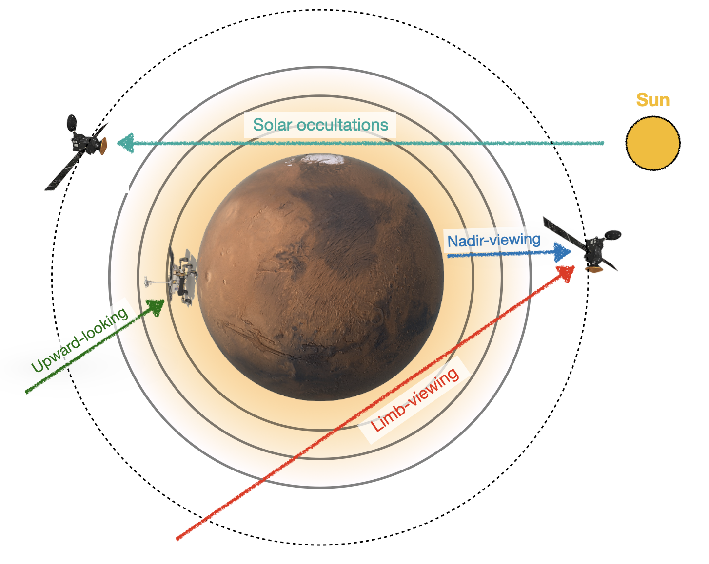
Remote sensing of planetary atmospheres can be mainly performed using three kinds of observations: nadir-viewing, limb-viewing and solar or stelar occultations. In addition, recent measurements of planetary atmospheres also include upward-looking measurements by instruments on the surface. NEMESIS can model the electromagnetic spectrum in any of these types of observations, but the fields of the Measurement class must be filled accordingly to set up the correct geometry. In this section, we provide examples of .spx or HDF5 input files for these different kinds of observations.

Nadir-viewing observations: single point measurements

Nadir-viewing observations are those in which the instruments observes straight down to the planet. Depending on the observation and the field-of-view (FOV) of the instrument, the spectra may represent just a single point of the planet, while the FOV of other measurements might encompass a large fraction or even the whole planet.

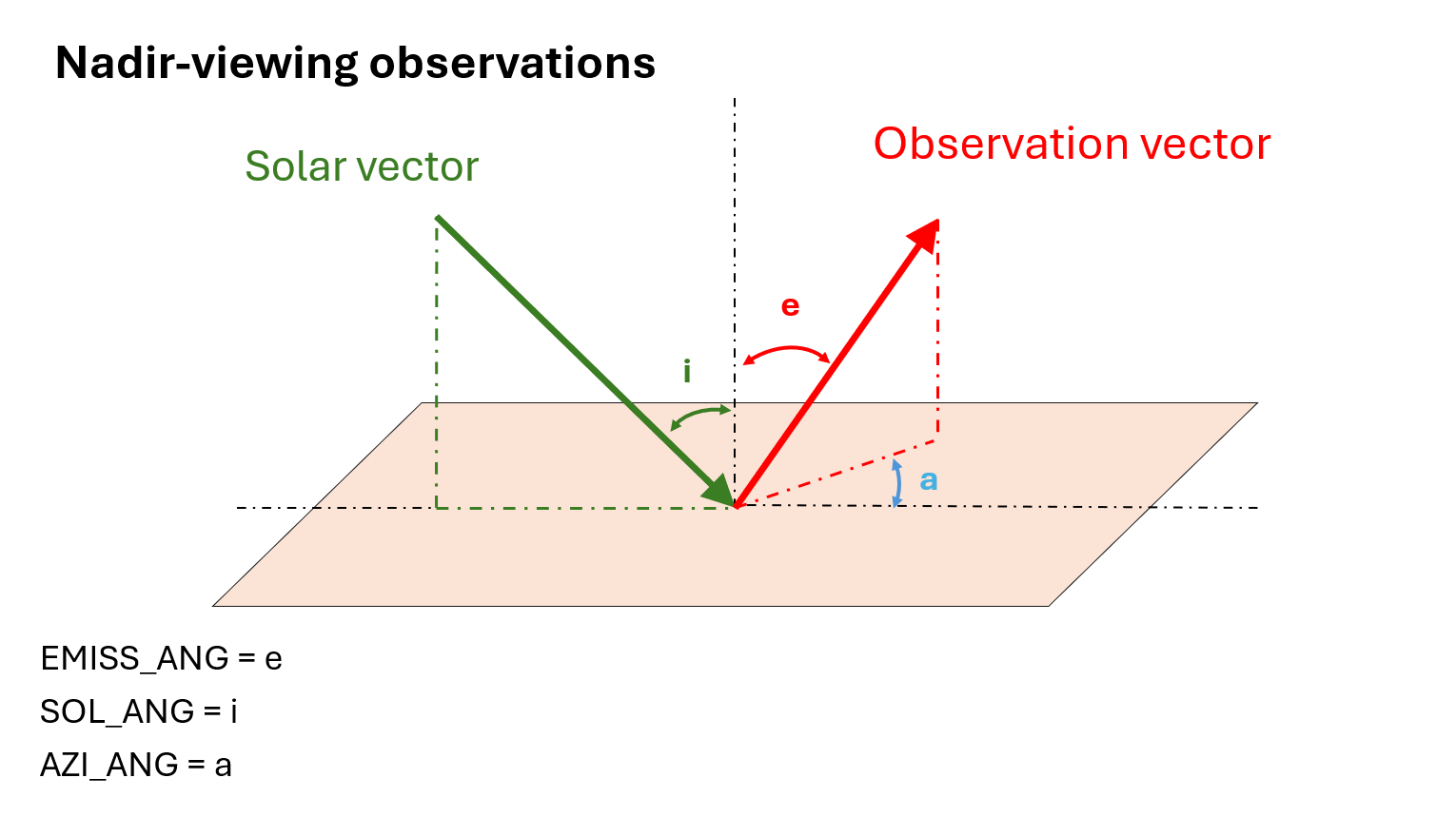
In the simplest case, where the measurement just corresponds to a single point on the planet, the main parameters describing the geometry are:

• FLAT and FLON represent the latitude and longitude of the sub-observer point on the planet.

• EMISS_ANG is the emission angle, defined as represented in the figure below.

• SOL_ANG is the solar zenith angle, defined as represented in the figure below.

• EMISS_ANG is the azimuth angle between the solar and observer vectors, defined as represented in the figure below. An azimuth angle of 0 degrees represents forward scattering, while an azimuth angle of 180 degrees represents backward scattering.

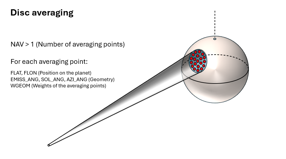
Nadir-viewing observations: disc averaging

There can be cases when the FOV of the instrument for a given measurement encompasses a relatively large portion of the planet disc, where the viewing geometry and the atmospheric properties may change. In those cases, we may need to compute several forward models and combine them to reconstruct the FOV. archNEMESIS can model this situation by allowing the definition of a number of averaging points (NAV), where several points in the FOV can be specified and later averaged later on. In particular, the FOV is reconstructed by using a weighted average, where each of the averaging points is given a particular weight (WGEOM).

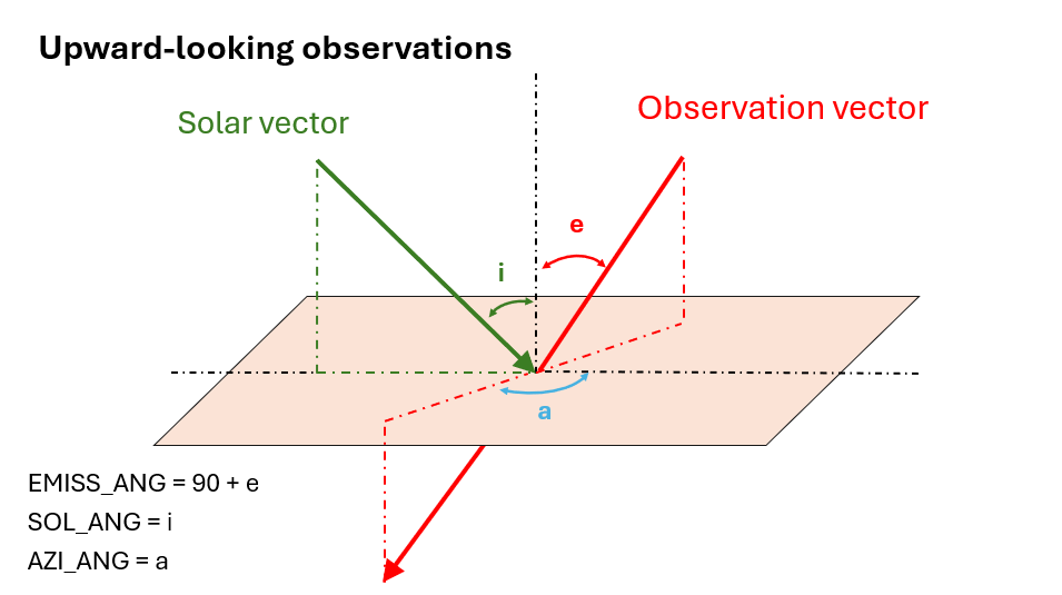
Upward-looking observations

archNEMESIS can also model the spectrum of a planetary atmosphere from an observer standing on the surface of the planet and looking at some point of the sky. This kind of geometry can be specified by setting the correct geometry in the atmosphere. In particular, the only difference with respect to the nadir-viewing observations resides in the definition of the emission angle. In particular, for an upward-looking observation, the emission angle needs to be defined as EMISS_ANG > 90, as indicated in the figure below.

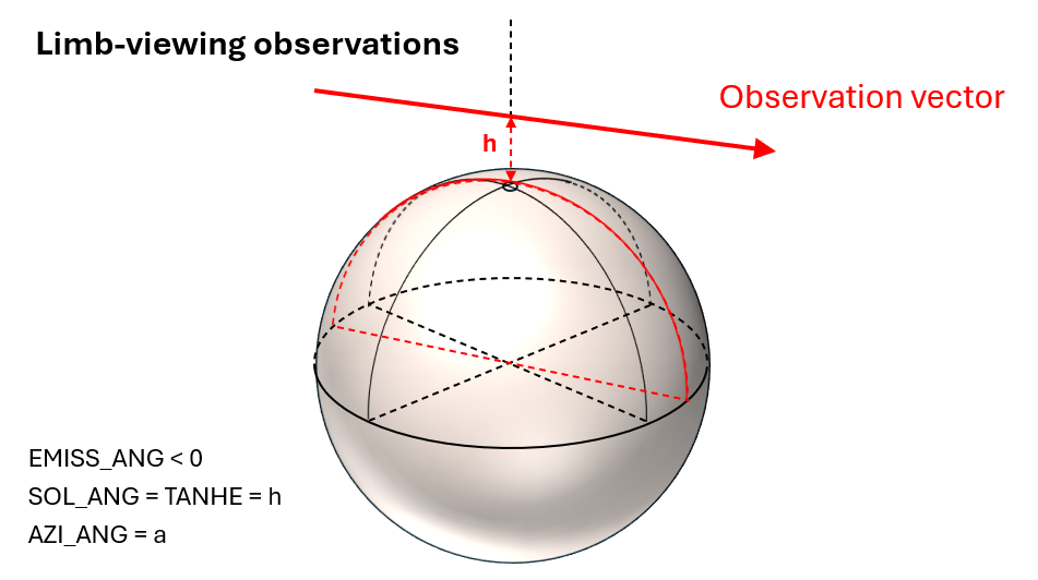
Limb-viewing observations

Instead of looking directly towards the surface, measurements of the planet’s limb may be performed. In order to specify this kind of geometry in archNEMESIS, the emission angle EMISS_ANG needs to be negative. In this case, the position of the SOL_ANG parameter in the .spx is changed by the tangent height of the measurement TANHE.