Introduction

The forward model refers to the set of functions in which the electromagnetic spectrum of a planetary atmosphere is calculated based on the information from the reference classes and the selected model parameterisations. In archNEMESIS, all these functions are implemented in the ForwardModel class. In essence, the inputs of the ForwardModel class are the reference classes and the Variables class, and the information within this class is used to perform the radiative transfer calculations and calculate the spectra.

For the users, running a forward model with archNEMESIS is relatively easy, given the information in the input reference classes is appropriately defined.

import archnemesis as ans

#Reading the input information from the HDF5 file
Atmosphere,Measurement,Spectroscopy,Scatter,Stellar,Surface,CIA,Layer,Variables,Retrieval,Telluric = ans.Files.read_input_files_hdf5(runname)

#Initialising ForwardModel class and feeding reference classes as input information
ForwardModel = ans.ForwardModel_0(Atmosphere=Atmosphere,Surface=Surface,Measurement=Measurement,Spectroscopy=Spectroscopy,Stellar=Stellar,Scatter=Scatter,CIA=CIA,Layer=Layer,Variables=Variables,Telluric=Telluric)

#Calculating forward model
SPECONV = ForwardModel.nemesisfm()

We recommend users to check the Examples to see how this forward model can be applied in practice.

Structure

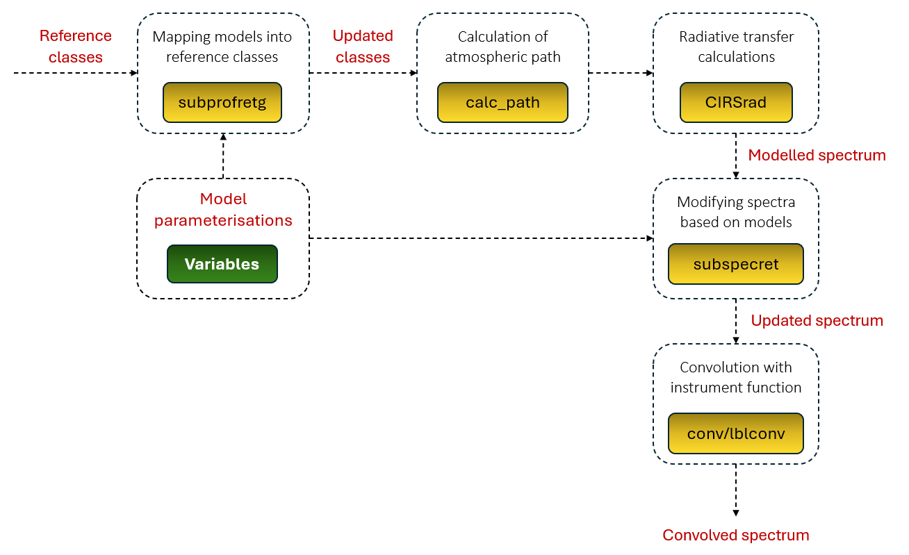
The figure below shows a sketch of the most relevant functions within the standard forward model implementation in archNEMESIS (i.e., ForwardModel.nemesisfm). As mentioned before, the inputs of the ForwardModel class are the reference classes and the model parameterisations, which are fed into the subprofretg method of this class. In this function, the reference classes are modified based on the selected model parameterisations, and the updated information is returned. After this, the calc_path method of the ForwardModel class splits the atmosphere into a finite number of layers and the atmospheric paths are calculated based on the geometry of the observation. CIRSrad is the main method where the radiative transfer calculations are performed, first calculating the relevant optical properties of each layer (e.g., absorption and scattering optical depths), calculating the internal radiation field if required, and finally calculating the electromagnetic spectrum of the planet given by our observing geometry. After the spectrum has been calculated, the subspecret method is in charge of modifying this modelled spectrum based on any relevant model parameterisations that might be added to mimic some instrument characteristics. Finally, the updated spectrum is convolved with the instrument lineshape to account for the spectral resolution of the instrument.

Typically, users of archNEMESIS will not generally need to modify most of these functions. The model parameterisations are implemented in subprofretg and subspecret, and users might want to familiarise with these two routines in case new parameterisations need to be added to the code for their specific use.

Drawing

Jacobian matrix

The Jacobian matrix is the matrix holding the information about the partial derivatives of the spectrum with respect to the model parameters. The information in this matrix is essential to perform retrievals using the optimal estimation framework, but also provide very useful diagnostic information about the sensitivity of the spectrum to certain atmospheric or surface properties.

In archNEMESIS, the Jacobian matrix can be calculated either analytically (in cases of non-scattering calculations), or numerically. The choice of calculating the derivatives analytically or numerically is automatically setup by the code using the Variables.INUM flag for each model parameter. When calculating the Jacobian matrix numerically, the forward models are simulated in parallel to increase the speed of the calculations.

The Jacobian matrix can be easily calculated with archNEMESIS by using the following code:

import archnemesis as ans

#Reading the input information from the HDF5 file
Atmosphere,Measurement,Spectroscopy,Scatter,Stellar,Surface,CIA,Layer,Variables,Retrieval,Telluric = ans.Files.read_input_files_hdf5(runname)

#Initialising ForwardModel class and feeding reference classes as input information
ForwardModel = ans.ForwardModel_0(Atmosphere=Atmosphere,Surface=Surface,Measurement=Measurement,Spectroscopy=Spectroscopy,Stellar=Stellar,Scatter=Scatter,CIA=CIA,Layer=Layer,Variables=Variables,Telluric=Telluric)

#Calculating Jacobian Matrix
YN,KK = ForwardModel.jacobian_nemesis()

Special cases

In certain cases, the radiative transfer calculations can be optimised so that computations are not unnecessarily repeated. This is typically the case when observing the same atmospheric column in different geometries for example, were most of the calculations can be performed only once (e.g., optical depths in each atmospheric layer will be the same), and only the final calculation of the specific geometry needs to be separate. In archNEMESIS, there are currently two alternative forward models that take advantage of these optimisations, which are explained in the following. In the future, new optimisations of the forward model can be introduced based on users needs.

nemesisSO

This option of the forward model is optimised for solar occulation observations. In these observations, the atmosphere is assumed to be spherically symmetric and it is observed at a set of different tangent heights through the limb. In this case, all geometries can be calculated simultaneously and the speed of the calculations is substantially increased. This option is only currently available for calculating atmospheric transmissions through the limb, but thermal emission calculations can be easily introduced if needed by the users.

A forward model of this type, as well as the calculation of the Jacobian matrix, can be easily run by using the following code.

import archnemesis as ans

#Reading the input information from the HDF5 file
Atmosphere,Measurement,Spectroscopy,Scatter,Stellar,Surface,CIA,Layer,Variables,Retrieval,Telluric = ans.Files.read_input_files_hdf5(runname)

#Initialising ForwardModel class and feeding reference classes as input information
ForwardModel = ans.ForwardModel_0(Atmosphere=Atmosphere,Surface=Surface,Measurement=Measurement,Spectroscopy=Spectroscopy,Stellar=Stellar,Scatter=Scatter,CIA=CIA,Layer=Layer,Variables=Variables,Telluric=Telluric)

#Calculating forward model
SPECONV = ForwardModel.nemesisSOfm()

#Calculating the Jacobian Matrix
YN,KK = ForwardModel.jacobian_nemesis(nemesisSO=True)

In addition, we recommend the users to check the Examples for getting insight of the kind of simulations performed in this mode.

nemesisC

In some cases, we may assume that the same atmospheric column is observed from a variety of geometries. This may be for example if observing the same atmospheric column from different spacecraft, or when we can assume that the atmosphere is symmetric in some region (e.g., latitudinally-symmetric). Similarly, when performing observations when surface-based instrumentation, the same atmosphere may be observed at different angles. In these situations, the speed of the calculations can be substantially increased by solving the radiative transfer equation generally and only separating the geometries at the end. This is particularly true when computing forward models in a multiple scattering scenario, when the internal radiation field of the atmosphere in all directions must be calculated regardless of whether we are modelling one or multiple geometries.

We introduced the forward model variation nemesisC, that essentially allows the calculation of multiple geometries under multiple scattering conditions. The only limitation is that all geometries must be either nadir-viewing (i.e., 0 \(\geq\) EMISS_ANG < 90) or upward-looking (i.e., 90 < EMISS_ANG \(\leq\) 180).

This forward model variation can be run by using the code below.

import archnemesis as ans

#Reading the input information from the HDF5 file
Atmosphere,Measurement,Spectroscopy,Scatter,Stellar,Surface,CIA,Layer,Variables,Retrieval,Telluric = ans.Files.read_input_files_hdf5(runname)

#Initialising ForwardModel class and feeding reference classes as input information
ForwardModel = ans.ForwardModel_0(Atmosphere=Atmosphere,Surface=Surface,Measurement=Measurement,Spectroscopy=Spectroscopy,Stellar=Stellar,Scatter=Scatter,CIA=CIA,Layer=Layer,Variables=Variables,Telluric=Telluric)

#Calculating forward model
SPECONV = ForwardModel.nemesisCfm()