Spectroscopic line data

ArchNEMESIS includes a reference class to operate with spectroscopic line data from databases such as HITRAN. Specifically, the attributes of the LineData class include the information required to calculate the line-by-line cross sections at arbitrary pressures and temperatures (e.g., line strengths, broadening coefficiencts, partition functions, etc).

In this notebook, we provide some examples showing how archNEMESIS can be used to process the spectroscopic line data.

import archnemesis as ans
import matplotlib.pyplot as plt
import numpy as np

1. Initialising the LineData class

In archNEMESIS, the functionality to process the spectroscopic line data is included in the LineData_0() class. This class has four main attributes that must be indicated when initialising the class:

• ID: Radtran ID of the gas we want to process.

• ISO: Radtran ID of the isotope we want to process.

• LINE_DATABASE : String containing the path to the HDF5 file where the line data is stored.

• PARTITION_FUNCTION_DATABASE : String containing the path to the HDF5 file where the partition function data is stored.

To perform calculations, archNEMESIS reads the line and partition function data from a HDF5 written with a custom format specific to this code. Generally, we aim to provide these files for standard databases such as HITRAN and store them in a public repository. For other line data sources, please contact the developers to help you create your own line data file readable by archNEMESIS.

The data files used in this notebook, corresponding to HITRAN24, can be downloaded following this link.

# Inputs are RADTRAN ID numbers
gas_id = ans.enum.GasEnum.CO
iso_id = 0

# Create LineData_0 instance
LineData = ans.LineData_0(
    gas_id, iso_id,
    LINE_DATABASE = ans.Data.path_data.archnemesis_resolve_path("/srv/workspace/data/nemesis/spectroscopy/linedata/hitran24/hitran24.h5"),
    PARTITION_FUNCTION_DATABASE = ans.Data.path_data.archnemesis_resolve_path("/srv/workspace/data/nemesis/spectroscopy/linedata/tips/tips2025.h5"),
)

print(f'{LineData._ans_database.LINE_DATABASE=}')

LineData._ans_database.LINE_DATABASE='/srv/workspace/data/nemesis/spectroscopy/linedata/hitran24/hitran24.h5'

2. Loading line data

Once the class has been initialised, it can be used to load the desired data into the class, so that we can perform calculations with it. The main function for reading the data is the fetch_linedata() method of the class.

When using this function, the method will load the required line data from the HDF5 file into the class and will store it in the LineData.line_data dictionary. This dictionary includes the following information:

• line_data[“RT_GAS_DESC”] : Indicates the gasID and isoID corresponding to each of the transitions. For cases when iso_id > 0 this will always be the same for all transitions, but in the case that we selected iso_id = 0, this descriptor provides information about the isotope the transition corresponds to.

• line_data[“NU”] : Wavenumber of each of the transitions (cm\(^{-1}\)).

• line_data[“SW”] : Line strength of the transition (cm\(^{-1}\) / (molec cm\(^{-2}\))).

• line_data[“A”] : Einstein A coeifficient (s\(^{-1}\)).

• line_data[“GAMMA_AMB”] : Ambient gas broadening coefficient (cm\(^{-1}\) atm\(^{-1}\)).

• line_data[“N_AMB”] : Temperature dependent exponent for “GAMMA_AMB”.

• line_data[“DELTA_AMB”] : Ambient gas pressure induced line-shift (cm\(^{-1}\) atm\(^{-1}\)).

• line_data[“GAMMA_SELF”] : Self-broadening coefficient (cm\(^{-1}\) atm\(^{-1}\)).

• line_data[“ELOWER”] : Lower state energy (cm\(^{-1}\)).

A more detailed explanation of these parameters can be found in the HITRAN website.

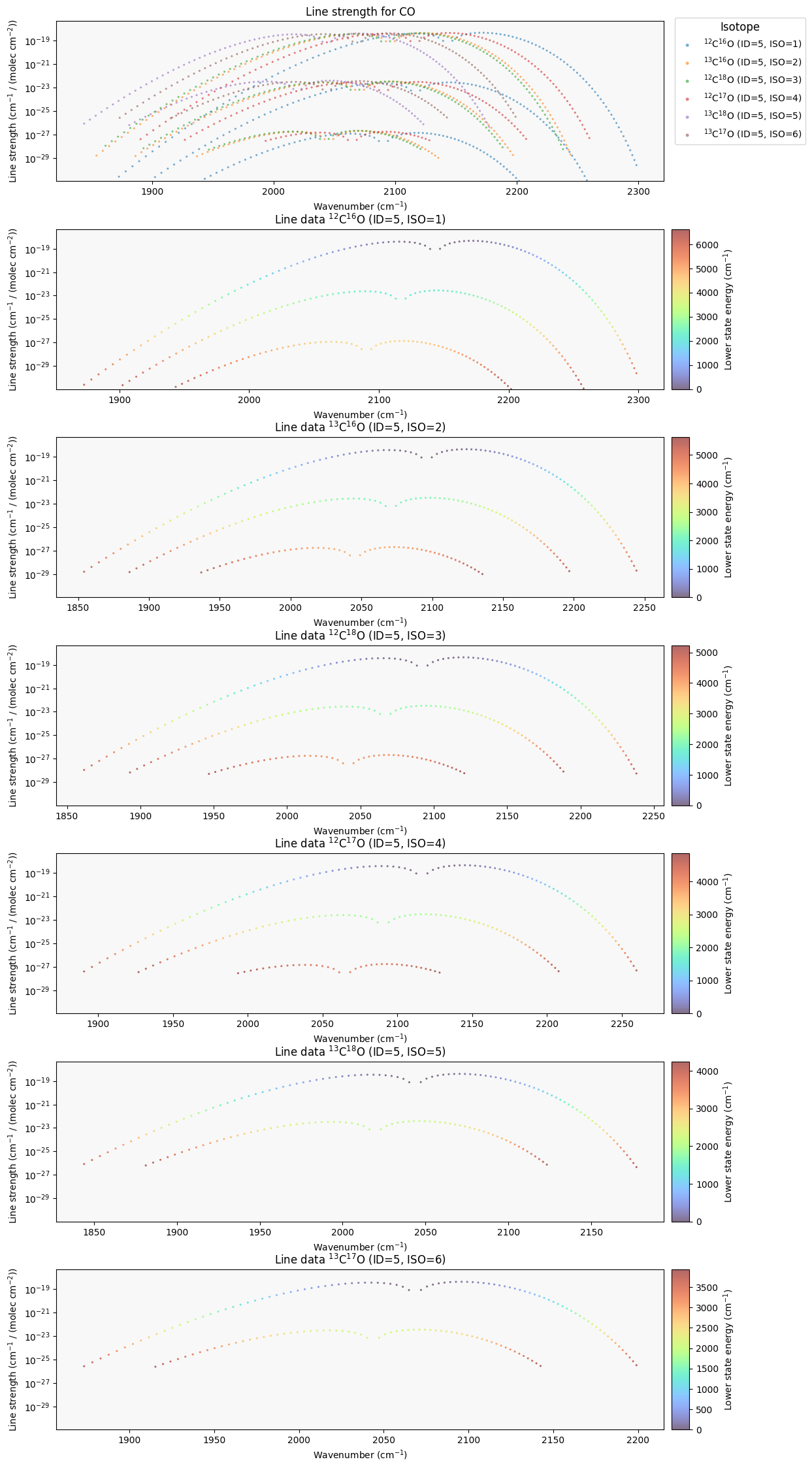
Once the data is loaded, it can be easily explored by printing the values in the dictionary. Similarly, the LineData class includes a method to create some diagnostic plots.

# Download line data for a specified spectral range
vmin = 1700.0
vmax = 2300.0
wave_unit = 0 #0 - Wavenumber (cm-1) ; 1 = Wavelength (um)
LineData.set_params(vmin=vmin, vmax=vmax, wave_unit=wave_unit).fetch_linedata()

LineData_0::fetch_partition_fn()
Actually getting the partition function

LineData_0(MEM=127031570341136,ID=5,ISO=0,params=LineDataParams(ambient_gasses=(<AmbientGasEnum.AIR: 0>,), wn_min=1700.0, wn_max=2300.0, s_min=-1, t_req=296, p_req=1, default_continuum_wn_bin_width=1.0))

#Printing some values
print("")
print("Content of line_data")
print(LineData.combined_line_data.RT_GAS_DESC.T)
print(LineData.combined_line_data.SW.T)
print("")
print("")

INFO :: create_from :: LineData_0.py-1051 :: iso_line_data._data.shape=(11, 279)
INFO :: create_from :: LineData_0.py-1051 :: iso_line_data._data.shape=(11, 252)
INFO :: create_from :: LineData_0.py-1051 :: iso_line_data._data.shape=(11, 238)
INFO :: create_from :: LineData_0.py-1051 :: iso_line_data._data.shape=(11, 215)
INFO :: create_from :: LineData_0.py-1051 :: iso_line_data._data.shape=(11, 169)
INFO :: create_from :: LineData_0.py-1051 :: iso_line_data._data.shape=(11, 158)

Content of line_data
[[5 1]
 [5 1]
 [5 1]
 ...
 [5 6]
 [5 6]
 [5 6]]
[2.56664977e-31 7.17486062e-31 1.96958946e-30 ... 1.48547919e-25
 7.01839303e-26 3.25750242e-26]

# Create diagnotic plots
LineData.plot_linedata(scatter_style_kw={'s':20})

/home/alday/Documents/Projects/archnemesis-dist/archnemesis/LineData_0.py:2562: UserWarning: This figure includes Axes that are not compatible with tight_layout, so results might be incorrect.
  plt.tight_layout()

3. Calculate the absorption cross sections

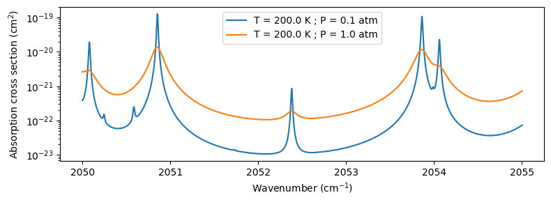
Apart from allowing the investigation of the line data, the LineData class includes some functionality to calculate the absorption cross following the formalism indicated in the HITRAN website.

The main method to perform these calculations is LineData.calculate_monochromatic_absorption(). This has several inputs that are important to specify:

• waves : Array of wavenumbers (\(cm^{-1}\)) or wavelengths (\(\mu\)) at which to calculate the absorption coefficient.

• temp : Ambient temperature (K).

• press : Ambient pressure (atm).

• amb_frac : Fraction of ambient pressure (1.0 = complete foreign broadening ; 0.0 = complete self broadening)

• wave_unit : Unit of the spectral array (0 = wavenumber in \(cm^{-1}\); 1 = wavelength in \(\mu\)m). Default = 0.

• lineshape_fn : This needs to point to one of the lineshapes stored in archnemesis.Data.lineshapes. Default = Data.lineshapes.voigt (Voigt profile).

• line_calculation_wavenumber_window : Wavenumber window around a line where the contribution from that line is considered (\(cm^{-1}\)). Default = 25 \(cm^{-1}\).

• line_strength_cutoff : Strength below which a line is ignored. Default = \(10^{-32}\).

• isotopic_abundances : If not None, use these abundances for each isotopologue instead of the default terrestrial ones.

It must be noted that, unlike NEMESIS conventions, the absorption coefficient calculated here MUST NOT be multiplied by a factor of \(10^{-20}\) as is is already expressed it in cm\(^{2}\).

wave_unit = 0     #0 - Wavenumber (cm-1) ; 1 = Wavelength (um)
waves = np.arange(2050,2055,0.0001)  #Wavenumber array

amb_frac = 1.0   #Fraction of ambient pressure (1.0 = complete foreign broadening ; 0.0 = complete self broadening)

temp1 = 200.      #Temperature (K)
press1 = 0.1      #Pressure (atm)
k1 = LineData.calculate_monochromatic_absorption(waves,temp1,press1,amb_frac,wave_unit=wave_unit,include_pressure_shift=True)

temp2 = 200.      #Temperature (K)
press2 = 1.0      #Pressure (atm)
k2 = LineData.calculate_monochromatic_absorption(waves,temp2,press2,amb_frac,wave_unit=wave_unit)

fig,ax1 = plt.subplots(1,1,figsize=(8,3))
ax1.plot(waves,k1,label=f"T = {temp1} K ; P = {press1} atm")
ax1.plot(waves,k2,label=f"T = {temp2} K ; P = {press2} atm")
ax1.set_yscale("log")
ax1.legend()
ax1.set_xlabel("Wavenumber (cm$^{-1}$)")
ax1.set_ylabel("Absorption cross section (cm$^2$)")
plt.tight_layout()