Exoplanets: primary transit

In this example, we show how archNEMESIS can be used to perform a retrieval of an exoplanet atmosphere through the analysis of transit observations. Specifically, in this example we are first going to generate a synthetic spectrum, and then retrieve the abundance of SO\(_2\) from the spectra, simulating how we would analyse a measured spectrum from an observatory.

The information about the reference classes here is obtained from an input HDF5 file with relevant information for the observation. This file can be easily generated following this tutorial.

[1]:

import archnemesis as ans
import numpy as np
import matplotlib.pyplot as plt

1. Generating the synthetic spectrum

In this example, we are going to read the information from the input file. However, we are going to modify the amount of SO\(_2\) to generate the synthetic spectrum, to see whether we can then recover it when performing the retrieval.

1.1. Reading the input file

[2]:

runname = "wasp-39b"

#Reading the input files
Atmosphere,Measurement,Spectroscopy,Scatter,Stellar,Surface,CIA,Layer,Variables,Retrieval,Telluric = ans.Files.read_input_files_hdf5(runname)

WARNING :: read_hdf5 :: Layer_0.py-379 :: When reading file "wasp-39b.h5", could not find element "Layer/BASEH" setting returned value to "None"
WARNING :: read_hdf5 :: Layer_0.py-380 :: When reading file "wasp-39b.h5", could not find element "Layer/BASEP" setting returned value to "None"
WARNING :: read_hdf5 :: Layer_0.py-381 :: When reading file "wasp-39b.h5", could not find element "Layer/TAUTOT" setting returned value to "None"
WARNING :: read_header :: Spectroscopy_0.py-566 :: self.NGAS=8 self.LOCATION=PathRedirectList(['/exomars/retrievals/nemesis/spectroscopy/Ktables/Exoplanets/Jake/R1000/H2O_R1000.kta', '/exomars/retrievals/nemesis/spectroscopy/Ktables/Exoplanets/Jake/R1000/CO2_R1000.kta', '/exomars/retrievals/nemesis/spectroscopy/Ktables/Exoplanets/Jake/R1000/CO_R1000.kta', '/exomars/retrievals/nemesis/spectroscopy/Ktables/Exoplanets/Jake/R1000/NH3_R1000.kta', '/exomars/retrievals/nemesis/spectroscopy/Ktables/Exoplanets/Jake/R1000/CH4_R1000.kta', '/exomars/retrievals/nemesis/spectroscopy/Ktables/Exoplanets/Jake/R1000/SO2_R1000.kta', '/exomars/retrievals/nemesis/spectroscopy/Ktables/Exoplanets/Jake/R1000/H2S_R1000.kta', '/exomars/retrievals/nemesis/spectroscopy/Ktables/Exoplanets/Jake/R1000/HCN_R1000.kta'], redirects = {})
INFO :: read_apr :: Variables_0.py-823 ::
Variables_0 :: read_apr :: varident [9 0 0]. Constructed model "Model0" (id=0)
INFO :: read_apr :: Variables_0.py-826 ::   Model0:
  |- id : 0
  |- parent classes: PreRTModelBase
  |- description: In this model, the atmospheric parameters are modelled as
  |               continuous profiles in which each element of the state vector
  |               corresponds to the atmospheric profile  at each altitude level
  |- n_state_vector_entries : 150
  |- state_vector_slice : slice(0, 150, None)
  |- state_vector_start : 0
  |- target : 0
  |- Parameters:
  |  |- full_profile :
  |  |  |- slice : slice(None, None, None)
  |  |  |- unit : PROFILE_TYPE
  |  |  |- description: Every value for each level of the profile
  |  |  |- apriori value : [1.e-06 1.e-06 1.e-06 1.e-06 1.e-06 1.e-06 1.e-06 1.e-06 1.e-06 1.e-06
   1.e-06 1.e-06 1.e-06 1.e-06 1.e-06 1.e-06 1.e-06 1.e-06 1.e-06 1.e-06
   1.e-06 1.e-06 1.e-06 1.e-06 1.e-06 1.e-06 1.e-06 1.e-06 1.e-06 1.e-06
   1.e-06 1.e-06 1.e-06 1.e-06 1.e-06 1.e-06 1.e-06 1.e-06 1.e-06 1.e-06
   1.e-06 1.e-06 1.e-06 1.e-06 1.e-06 1.e-06 1.e-06 1.e-06 1.e-06 1.e-06
   1.e-06 1.e-06 1.e-06 1.e-06 1.e-06 1.e-06 1.e-06 1.e-06 1.e-06 1.e-06
   1.e-06 1.e-06 1.e-06 1.e-06 1.e-06 1.e-06 1.e-06 1.e-06 1.e-06 1.e-06
   1.e-06 1.e-06 1.e-06 1.e-06 1.e-06 1.e-06 1.e-06 1.e-06 1.e-06 1.e-06
   1.e-06 1.e-06 1.e-06 1.e-06 1.e-06 1.e-06 1.e-06 1.e-06 1.e-06 1.e-06
   1.e-06 1.e-06 1.e-06 1.e-06 1.e-06 1.e-06 1.e-06 1.e-06 1.e-06 1.e-06
   1.e-06 1.e-06 1.e-06 1.e-06 1.e-06 1.e-06 1.e-06 1.e-06 1.e-06 1.e-06
   1.e-06 1.e-06 1.e-06 1.e-06 1.e-06 1.e-06 1.e-06 1.e-06 1.e-06 1.e-06
   1.e-06 1.e-06 1.e-06 1.e-06 1.e-06 1.e-06 1.e-06 1.e-06 1.e-06 1.e-06
   1.e-06 1.e-06 1.e-06 1.e-06 1.e-06 1.e-06 1.e-06 1.e-06 1.e-06 1.e-06
   1.e-06 1.e-06 1.e-06 1.e-06 1.e-06 1.e-06 1.e-06 1.e-06 1.e-06 1.e-06]

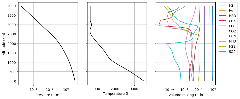
[3]:

Atmosphere.plot_Atm()

../../_images/examples_retrieval_exoplanet_transit_retrieval_exoplanet_5_0.png

1.2. Modifying the amount of SO\(_2\)

To modify the amount of SO\(_2\) in the atmosphere, we are going to write a new .apr file, so that the reference classes are updated when computing the forward model

[4]:

#Writing new .apr file
nvar = 1
varident = np.zeros((3,nvar),dtype="int32")
varident[:,0] = [9,0,2]   #I1=9 (SO2); I2=0 (All isotopes); I3=0 (Model 2 - scaling factor)
fapr = open(runname+".apr","w")
fapr.write("#Synthetic retrieval for exoplanet primary transit \n")
fapr.write("\t %i \n" % (nvar))
fapr.write("\t %i \t %i \t %i \n" % (varident[0,0],varident[1,0],varident[2,0]))
fapr.write("1.0 0.1 \n")
fapr.close()

[5]:

#Reading the input files
Atmosphere,Measurement,Spectroscopy,Scatter,Stellar,Surface,CIA,Layer,Variables,Retrieval,Telluric = ans.Files.read_input_files_hdf5(runname)

WARNING :: read_hdf5 :: Layer_0.py-379 :: When reading file "wasp-39b.h5", could not find element "Layer/BASEH" setting returned value to "None"
WARNING :: read_hdf5 :: Layer_0.py-380 :: When reading file "wasp-39b.h5", could not find element "Layer/BASEP" setting returned value to "None"
WARNING :: read_hdf5 :: Layer_0.py-381 :: When reading file "wasp-39b.h5", could not find element "Layer/TAUTOT" setting returned value to "None"
WARNING :: read_header :: Spectroscopy_0.py-566 :: self.NGAS=8 self.LOCATION=PathRedirectList(['/exomars/retrievals/nemesis/spectroscopy/Ktables/Exoplanets/Jake/R1000/H2O_R1000.kta', '/exomars/retrievals/nemesis/spectroscopy/Ktables/Exoplanets/Jake/R1000/CO2_R1000.kta', '/exomars/retrievals/nemesis/spectroscopy/Ktables/Exoplanets/Jake/R1000/CO_R1000.kta', '/exomars/retrievals/nemesis/spectroscopy/Ktables/Exoplanets/Jake/R1000/NH3_R1000.kta', '/exomars/retrievals/nemesis/spectroscopy/Ktables/Exoplanets/Jake/R1000/CH4_R1000.kta', '/exomars/retrievals/nemesis/spectroscopy/Ktables/Exoplanets/Jake/R1000/SO2_R1000.kta', '/exomars/retrievals/nemesis/spectroscopy/Ktables/Exoplanets/Jake/R1000/H2S_R1000.kta', '/exomars/retrievals/nemesis/spectroscopy/Ktables/Exoplanets/Jake/R1000/HCN_R1000.kta'], redirects = {})
INFO :: read_apr :: Variables_0.py-823 ::
Variables_0 :: read_apr :: varident [9 0 2]. Constructed model "Model2" (id=2)
INFO :: read_apr :: Variables_0.py-826 ::   Model2:
  |- id : 2
  |- parent classes: PreRTModelBase
  |- description: In this model, the atmospheric parameters are scaled using a
  |               single factor with  respect to the vertical profiles in the
  |               reference atmosphere
  |- n_state_vector_entries : 1
  |- state_vector_slice : slice(0, 1, None)
  |- state_vector_start : 0
  |- target : 0
  |- Parameters:
  |  |- scaling_factor :
  |  |  |- slice : slice(0, 1, None)
  |  |  |- unit : PROFILE_TYPE
  |  |  |- description: Scaling factor applied to the reference profile
  |  |  |- apriori value : 1.0

1.2. Generating a forward model

[6]:

ForwardModel = ans.ForwardModel_0(Atmosphere=Atmosphere,Surface=Surface,Measurement=Measurement,Spectroscopy=Spectroscopy,Stellar=Stellar,Scatter=Scatter,CIA=CIA,Layer=Layer,Variables=Variables,Telluric=Telluric)

SPECONV = ForwardModel.nemesisPTfm()

INFO :: __init__ :: ForwardModel_0.py-256 :: Checking atmospheric gasses have spectroscopy data.
WARNING :: __init__ :: ForwardModel_0.py-303 :: Not all atmospheric gasses have spectroscopy data.
# WARNING #########################################################################

The following atmospheric gasses ARE NOT PRESENT in the spectroscopy data and WILL NOT CONTRIBUTE TO OPACITY:

    H2 (id 39) isotopologue 0
    He (id 40) isotopologue 0

To deactivate this warning place a path to a k-table file for these gasses in one of the following locations (depending upon your input file type):

    [HDF5 Input]
        In the "wasp121.h5" file, add an entry to "/Spectroscopy/LOCATION"
        and update "/Spectroscopy/NGAS" appropriately.

    [LEGACY Input]
        Add an entry to the "wasp121.kls" file.

# END WARNING #####################################################################
INFO :: nemesisPTfm :: ForwardModel_0.py-1809 :: Calculating forward model for primary transit observation
INFO :: nemesisPTfm :: ForwardModel_0.py-1837 :: Running CIRSrad for primary transit observation
INFO :: calculate_vertical_cia_opacity :: ForwardModel_0.py-3765 :: Calculating self.CIAX opacity
WARNING :: calc_tau_cia :: ForwardModel_0.py-4336 ::  in CIA :: Calculation wavelengths expand a larger range than in CIA table
INFO :: calculate_layer_opacity :: ForwardModel_0.py-3834 :: CIRSrad :: Aerosol optical depths at  (0.3001500070095062, ' :: ', array([0.]))
INFO :: calculate_layer_opacity :: ForwardModel_0.py-3852 :: Calculating TOTAL opacity
INFO :: calculate_layer_opacity :: ForwardModel_0.py-3869 :: CIRSradg :: Calculating TOTAL line-of-sight opacity
INFO :: CIRSrad :: ForwardModel_0.py-4201 :: CIRSrad :: IMODM = <PathCalc.PLANCK_FUNCTION_AT_BIN_CENTRE: 8192>
INFO :: nemesisPTfm :: ForwardModel_0.py-1890 :: Convolving spectra and gradients with instrument line shape

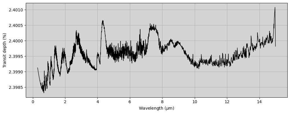
[7]:

fig,ax1 = plt.subplots(1,1,figsize=(10,4))

ax1.plot(Measurement.VCONV[:,0],SPECONV,c='black',linewidth=1.)
ax1.grid()
ax1.set_xlabel('Wavelength ($\mu$m)')
ax1.set_ylabel('Transit depth (%)')
ax1.set_facecolor('lightgray')
plt.tight_layout()

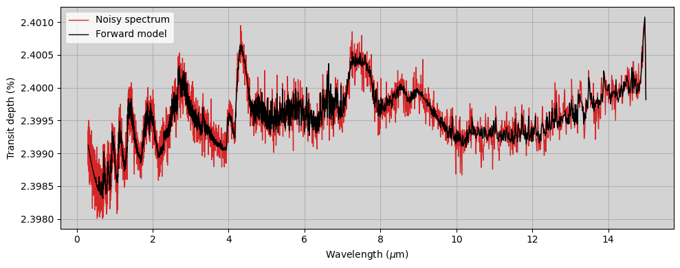
../../_images/examples_retrieval_exoplanet_transit_retrieval_exoplanet_11_0.png

1.3. Adding random noise to the spectrum

Now, we add some random noise to the spectrum. This will of course be dependent on the quality of the observation. Here, we are going to assume we have a 2\(\%\) error at all wavelengths.

[8]:

noise_level = 7.0e-5

noise = np.random.normal(loc=0.0,scale=noise_level * SPECONV[:,0])

synthetic_spectrum = (SPECONV.T + noise).T
synthetic_error = SPECONV * noise_level

fig,ax1 = plt.subplots(1,1,figsize=(10,4))

ax1.plot(Measurement.VCONV[:,0],synthetic_spectrum,c='tab:red',linewidth=1.,label="Noisy spectrum")
ax1.plot(Measurement.VCONV[:,0],SPECONV,c='black',linewidth=1.,label="Forward model")
ax1.grid()
ax1.legend()
ax1.set_xlabel('Wavelength ($\mu$m)')
ax1.set_ylabel('Transit depth (%)')
ax1.set_facecolor('lightgray')
plt.tight_layout()

../../_images/examples_retrieval_exoplanet_transit_retrieval_exoplanet_13_0.png

1.4. Re-writing file

Now we need to overwrite the Measurement class to include the measured spectrum and uncertainty in the input file.

[9]:

Measurement.edit_MEAS(synthetic_spectrum)
Measurement.edit_ERRMEAS(synthetic_error)

Measurement.write_hdf5(runname)

2. Running the retrieval

Now that we have a “measured” spectrum, we can perform a retrieval to see if we can recover a given atmospheric parameter. In our case, we are going to retrieve a continuous vertical profile of SO\(_2\). To do so, we are going to specify this information in the .apr file, and then we will perform the retrieval.

2.1. Writing .apr file

[10]:

def write_apr_continuous_profile(filename,press,profile,profile_err,clen=1.5):
    """
    Function to write the a priori file for the retrieval of a continuous vertical profile
    """

    #Write file
    fref = open(filename,'w')
    fref.write('\t %i \t %10.3f \n' % (len(press),clen))
    for i in range(len(press)):
        fref.write('\t %10.6e \t %10.6e \t %10.6e \n' % (press[i],profile[i],profile_err[i]))
    fref.close()


#Writing new .apr file
nvar = 1
varident = np.zeros((3,nvar),dtype="int32")
varident[:,0] = [9,0,0]   #I1=9 (SO2); I2=0 (All isotopes); I3=0 (Model 0 - continuous profile)
fapr = open(runname+".apr","w")
fapr.write("#Synthetic retrieval for exoplanet primary transit \n")
fapr.write("\t %i \n" % (nvar))
fapr.write("\t %i \t %i \t %i \n" % (varident[0,0],varident[1,0],varident[2,0]))
fapr.write("so2apr.dat \n")
fapr.close()

#Writing the so2apr.dat file
so2_apr = np.ones(Atmosphere.NP) * 1.0e-6
so2_aprerr = so2_apr * 0.5   #50% uncertainty
write_apr_continuous_profile("so2apr.dat",Atmosphere.P,so2_apr,so2_aprerr,clen=1.5)

2.2. Setting up retrieval

[11]:

Retrieval = ans.OptimalEstimation_0(IRET=0)

Retrieval.NITER = 5       #Number of iterations
Retrieval.PHILIMIT = 0.1   #Convergence criterion
Retrieval.NCORES = 1       #Number of available cores (not needed for this version of the forward model)

Retrieval.assess_input()
Retrieval.write_input_hdf5(runname)

2.3. Running retrieval

[12]:

legacy_files=False   #Reading the HDF5 file
retrieval_method=0   #Optimal Estimtion
NCores=None          #Since we are not including scattering in this calculation (Scatter.ISCAT=0), the Jacobian is calculated analytically
nemesisPT=True       #We indicate that the retrieval must be run using the primary transit forward model

ans.Retrievals.retrieval_nemesis(runname,legacy_files=legacy_files,retrieval_method=retrieval_method,NCores=NCores,nemesisPT=nemesisPT)

WARNING :: read_hdf5 :: Layer_0.py-379 :: When reading file "wasp-39b.h5", could not find element "Layer/BASEH" setting returned value to "None"
WARNING :: read_hdf5 :: Layer_0.py-380 :: When reading file "wasp-39b.h5", could not find element "Layer/BASEP" setting returned value to "None"
WARNING :: read_hdf5 :: Layer_0.py-381 :: When reading file "wasp-39b.h5", could not find element "Layer/TAUTOT" setting returned value to "None"
WARNING :: read_header :: Spectroscopy_0.py-566 :: self.NGAS=8 self.LOCATION=PathRedirectList(['/exomars/retrievals/nemesis/spectroscopy/Ktables/Exoplanets/Jake/R1000/H2O_R1000.kta', '/exomars/retrievals/nemesis/spectroscopy/Ktables/Exoplanets/Jake/R1000/CO2_R1000.kta', '/exomars/retrievals/nemesis/spectroscopy/Ktables/Exoplanets/Jake/R1000/CO_R1000.kta', '/exomars/retrievals/nemesis/spectroscopy/Ktables/Exoplanets/Jake/R1000/NH3_R1000.kta', '/exomars/retrievals/nemesis/spectroscopy/Ktables/Exoplanets/Jake/R1000/CH4_R1000.kta', '/exomars/retrievals/nemesis/spectroscopy/Ktables/Exoplanets/Jake/R1000/SO2_R1000.kta', '/exomars/retrievals/nemesis/spectroscopy/Ktables/Exoplanets/Jake/R1000/H2S_R1000.kta', '/exomars/retrievals/nemesis/spectroscopy/Ktables/Exoplanets/Jake/R1000/HCN_R1000.kta'], redirects = {})
INFO :: read_apr :: Variables_0.py-823 ::
Variables_0 :: read_apr :: varident [9 0 0]. Constructed model "Model0" (id=0)
INFO :: read_apr :: Variables_0.py-826 ::   Model0:
  |- id : 0
  |- parent classes: PreRTModelBase
  |- description: In this model, the atmospheric parameters are modelled as
  |               continuous profiles in which each element of the state vector
  |               corresponds to the atmospheric profile  at each altitude level
  |- n_state_vector_entries : 150
  |- state_vector_slice : slice(0, 150, None)
  |- state_vector_start : 0
  |- target : 0
  |- Parameters:
  |  |- full_profile :
  |  |  |- slice : slice(None, None, None)
  |  |  |- unit : PROFILE_TYPE
  |  |  |- description: Every value for each level of the profile
  |  |  |- apriori value : [1.e-06 1.e-06 1.e-06 1.e-06 1.e-06 1.e-06 1.e-06 1.e-06 1.e-06 1.e-06
   1.e-06 1.e-06 1.e-06 1.e-06 1.e-06 1.e-06 1.e-06 1.e-06 1.e-06 1.e-06
   1.e-06 1.e-06 1.e-06 1.e-06 1.e-06 1.e-06 1.e-06 1.e-06 1.e-06 1.e-06
   1.e-06 1.e-06 1.e-06 1.e-06 1.e-06 1.e-06 1.e-06 1.e-06 1.e-06 1.e-06
   1.e-06 1.e-06 1.e-06 1.e-06 1.e-06 1.e-06 1.e-06 1.e-06 1.e-06 1.e-06
   1.e-06 1.e-06 1.e-06 1.e-06 1.e-06 1.e-06 1.e-06 1.e-06 1.e-06 1.e-06
   1.e-06 1.e-06 1.e-06 1.e-06 1.e-06 1.e-06 1.e-06 1.e-06 1.e-06 1.e-06
   1.e-06 1.e-06 1.e-06 1.e-06 1.e-06 1.e-06 1.e-06 1.e-06 1.e-06 1.e-06
   1.e-06 1.e-06 1.e-06 1.e-06 1.e-06 1.e-06 1.e-06 1.e-06 1.e-06 1.e-06
   1.e-06 1.e-06 1.e-06 1.e-06 1.e-06 1.e-06 1.e-06 1.e-06 1.e-06 1.e-06
   1.e-06 1.e-06 1.e-06 1.e-06 1.e-06 1.e-06 1.e-06 1.e-06 1.e-06 1.e-06
   1.e-06 1.e-06 1.e-06 1.e-06 1.e-06 1.e-06 1.e-06 1.e-06 1.e-06 1.e-06
   1.e-06 1.e-06 1.e-06 1.e-06 1.e-06 1.e-06 1.e-06 1.e-06 1.e-06 1.e-06
   1.e-06 1.e-06 1.e-06 1.e-06 1.e-06 1.e-06 1.e-06 1.e-06 1.e-06 1.e-06
   1.e-06 1.e-06 1.e-06 1.e-06 1.e-06 1.e-06 1.e-06 1.e-06 1.e-06 1.e-06]
INFO :: coreretOE :: OptimalEstimation_0.py-1325 :: coreretOE :: Starting OptimalEstimation retrieval with NITER=5 PHILIMIT=0.1 NCORES=None
INFO :: coreretOE :: OptimalEstimation_0.py-1352 :: nemesis :: Calculating Jacobian matrix KK
INFO :: jacobian_nemesis :: ForwardModel_0.py-2191 :: Calculating analytical part of the Jacobian :: Calling nemesisfmg
INFO :: nemesisPTfm :: ForwardModel_0.py-1809 :: Calculating forward model for primary transit observation
INFO :: nemesisPTfm :: ForwardModel_0.py-1840 :: Running CIRSradg for primary transit observation
INFO :: calculate_vertical_cia_opacity :: ForwardModel_0.py-3765 :: Calculating self.CIAX opacity
WARNING :: calc_tau_cia :: ForwardModel_0.py-4336 ::  in CIA :: Calculation wavelengths expand a larger range than in CIA table
INFO :: calculate_layer_opacity :: ForwardModel_0.py-3834 :: CIRSrad :: Aerosol optical depths at  (0.3001500070095062, ' :: ', array([0.]))
INFO :: calculate_layer_opacity :: ForwardModel_0.py-3852 :: Calculating TOTAL opacity
INFO :: calculate_layer_opacity :: ForwardModel_0.py-3869 :: CIRSradg :: Calculating TOTAL line-of-sight opacity
INFO :: CIRSrad :: ForwardModel_0.py-4201 :: CIRSrad :: IMODM = <PathCalc.PLANCK_FUNCTION_AT_BIN_CENTRE: 8192>
INFO :: nemesisPTfm :: ForwardModel_0.py-1844 :: Mapping gradients from Layer to Profile
INFO :: nemesisPTfm :: ForwardModel_0.py-1856 :: Mapping gradients from Profile to State Vector
INFO :: nemesisPTfm :: ForwardModel_0.py-1890 :: Convolving spectra and gradients with instrument line shape
INFO :: coreretOE :: OptimalEstimation_0.py-1361 :: nemesis :: Calculating gain matrix
INFO :: coreretOE :: OptimalEstimation_0.py-1367 :: nemesis :: Calculating cost function
WARNING :: calc_phiret :: OptimalEstimation_0.py-629 :: calc_phiret: measurement_diff_cost=5263.76821817002, apriori_diff_cost=0.0, chisq=1.3448564686177875, measurement_diff_cost+apriori_diff_cost=5263.76821817002
INFO :: coreretOE :: OptimalEstimation_0.py-1371 :: chisq/ny = 1.3448564686177875
INFO :: coreretOE :: OptimalEstimation_0.py-1378 ::     iter | iter_state       | phi       | chisq     | state vector

INFO :: coreretOE :: OptimalEstimation_0.py-1379 ::     0000 | PHI INITIAL      | 5.264E+03 | 1.345E+00 | -1.382E+01 -1.382E+01 -1.382E+01 -1.382E+01 -1.382E+01 -1.382E+01 -1.382E+01 -1.382E+01 -1.382E+01 -1.382E+01 -1.382E+01 -1.382E+01 -1.382E+01 -1.382E+01 -1.382E+01 -1.382E+01 -1.382E+01 -1.382E+01 -1.382E+01 -1.382E+01 -1.382E+01 -1.382E+01 -1.382E+01 -1.382E+01 -1.382E+01 -1.382E+01 -1.382E+01 -1.382E+01 -1.382E+01 -1.382E+01 -1.382E+01 -1.382E+01 -1.382E+01 -1.382E+01 -1.382E+01 -1.382E+01 -1.382E+01 -1.382E+01 -1.382E+01 -1.382E+01 -1.382E+01 -1.382E+01 -1.382E+01 -1.382E+01 -1.382E+01 -1.382E+01 -1.382E+01 -1.382E+01 -1.382E+01 -1.382E+01 -1.382E+01 -1.382E+01 -1.382E+01 -1.382E+01 -1.382E+01 -1.382E+01 -1.382E+01 -1.382E+01 -1.382E+01 -1.382E+01 -1.382E+01 -1.382E+01 -1.382E+01 -1.382E+01 -1.382E+01 -1.382E+01 -1.382E+01 -1.382E+01 -1.382E+01 -1.382E+01 -1.382E+01 -1.382E+01 -1.382E+01 -1.382E+01 -1.382E+01 -1.382E+01 -1.382E+01 -1.382E+01 -1.382E+01 -1.382E+01 -1.382E+01 -1.382E+01 -1.382E+01 -1.382E+01 -1.382E+01 -1.382E+01 -1.382E+01 -1.382E+01 -1.382E+01 -1.382E+01 -1.382E+01 -1.382E+01 -1.382E+01 -1.382E+01 -1.382E+01 -1.382E+01 -1.382E+01 -1.382E+01 -1.382E+01 -1.382E+01 -1.382E+01 -1.382E+01 -1.382E+01 -1.382E+01 -1.382E+01 -1.382E+01 -1.382E+01 -1.382E+01 -1.382E+01 -1.382E+01 -1.382E+01 -1.382E+01 -1.382E+01 -1.382E+01 -1.382E+01 -1.382E+01 -1.382E+01 -1.382E+01 -1.382E+01 -1.382E+01 -1.382E+01 -1.382E+01 -1.382E+01 -1.382E+01 -1.382E+01 -1.382E+01 -1.382E+01 -1.382E+01 -1.382E+01 -1.382E+01 -1.382E+01 -1.382E+01 -1.382E+01 -1.382E+01 -1.382E+01 -1.382E+01 -1.382E+01 -1.382E+01 -1.382E+01 -1.382E+01 -1.382E+01 -1.382E+01 -1.382E+01 -1.382E+01 -1.382E+01 -1.382E+01 -1.382E+01 -1.382E+01 -1.382E+01 -1.382E+01

INFO :: assess :: OptimalEstimation_0.py-669 :: Assess:
INFO :: assess :: OptimalEstimation_0.py-670 :: Average of diagonal elements of Kk*Sx*Kt : 2.829731868459669e-08
INFO :: assess :: OptimalEstimation_0.py-671 :: Average of diagonal elements of Se : 2.8206673978263875e-08
INFO :: assess :: OptimalEstimation_0.py-672 :: Ratio = 1.003213590741066
INFO :: assess :: OptimalEstimation_0.py-673 :: Average of Kk*Sx*Kt/Se element ratio : 1.0032114546874633
INFO :: coreretOE :: OptimalEstimation_0.py-1405 :: nemesis :: Iteration 0/5
INFO :: coreretOE :: OptimalEstimation_0.py-1424 :: nemesis :: Calculating next iterated state vector
INFO :: coreretOE :: OptimalEstimation_0.py-1477 :: nemesis :: Calculating Jacobian matrix KK
INFO :: jacobian_nemesis :: ForwardModel_0.py-2191 :: Calculating analytical part of the Jacobian :: Calling nemesisfmg
INFO :: nemesisPTfm :: ForwardModel_0.py-1809 :: Calculating forward model for primary transit observation
INFO :: nemesisPTfm :: ForwardModel_0.py-1840 :: Running CIRSradg for primary transit observation
INFO :: calculate_vertical_cia_opacity :: ForwardModel_0.py-3765 :: Calculating self.CIAX opacity
WARNING :: calc_tau_cia :: ForwardModel_0.py-4336 ::  in CIA :: Calculation wavelengths expand a larger range than in CIA table
INFO :: calculate_layer_opacity :: ForwardModel_0.py-3834 :: CIRSrad :: Aerosol optical depths at  (0.3001500070095062, ' :: ', array([0.]))
INFO :: calculate_layer_opacity :: ForwardModel_0.py-3852 :: Calculating TOTAL opacity
INFO :: calculate_layer_opacity :: ForwardModel_0.py-3869 :: CIRSradg :: Calculating TOTAL line-of-sight opacity
INFO :: CIRSrad :: ForwardModel_0.py-4201 :: CIRSrad :: IMODM = <PathCalc.PLANCK_FUNCTION_AT_BIN_CENTRE: 8192>
INFO :: nemesisPTfm :: ForwardModel_0.py-1844 :: Mapping gradients from Layer to Profile
INFO :: nemesisPTfm :: ForwardModel_0.py-1856 :: Mapping gradients from Profile to State Vector
INFO :: nemesisPTfm :: ForwardModel_0.py-1890 :: Convolving spectra and gradients with instrument line shape
WARNING :: calc_phiret :: OptimalEstimation_0.py-629 :: calc_phiret: measurement_diff_cost=4204.170963217051, apriori_diff_cost=27.690697880571026, chisq=1.0741366794116125, measurement_diff_cost+apriori_diff_cost=4231.861661097622
INFO :: coreretOE :: OptimalEstimation_0.py-1500 :: chisq/ny = 1.0741366794116125
INFO :: coreretOE :: OptimalEstimation_0.py-1504 :: Successful iteration. Updating xn,yn and kk
WARNING :: calc_phiret :: OptimalEstimation_0.py-629 :: calc_phiret: measurement_diff_cost=4204.170963217051, apriori_diff_cost=27.690697880571026, chisq=1.0741366794116125, measurement_diff_cost+apriori_diff_cost=4231.861661097622
INFO :: coreretOE :: OptimalEstimation_0.py-1543 ::     iter | iter_state       | phi       | chisq     | state vector

INFO :: coreretOE :: OptimalEstimation_0.py-1544 ::     0000 | PHI REDUCED      | 4.232E+03 | 1.074E+00 | -1.381E+01 -1.381E+01 -1.381E+01 -1.381E+01 -1.381E+01 -1.381E+01 -1.381E+01 -1.381E+01 -1.380E+01 -1.380E+01 -1.380E+01 -1.380E+01 -1.380E+01 -1.380E+01 -1.379E+01 -1.379E+01 -1.379E+01 -1.379E+01 -1.378E+01 -1.378E+01 -1.378E+01 -1.377E+01 -1.377E+01 -1.376E+01 -1.376E+01 -1.375E+01 -1.374E+01 -1.373E+01 -1.373E+01 -1.372E+01 -1.370E+01 -1.369E+01 -1.368E+01 -1.366E+01 -1.365E+01 -1.363E+01 -1.361E+01 -1.359E+01 -1.356E+01 -1.354E+01 -1.350E+01 -1.347E+01 -1.343E+01 -1.339E+01 -1.335E+01 -1.330E+01 -1.324E+01 -1.318E+01 -1.311E+01 -1.304E+01 -1.296E+01 -1.288E+01 -1.280E+01 -1.270E+01 -1.261E+01 -1.251E+01 -1.242E+01 -1.233E+01 -1.222E+01 -1.213E+01 -1.206E+01 -1.198E+01 -1.191E+01 -1.185E+01 -1.180E+01 -1.177E+01 -1.175E+01 -1.174E+01 -1.174E+01 -1.175E+01 -1.178E+01 -1.181E+01 -1.185E+01 -1.190E+01 -1.195E+01 -1.201E+01 -1.207E+01 -1.214E+01 -1.220E+01 -1.227E+01 -1.234E+01 -1.241E+01 -1.247E+01 -1.254E+01 -1.260E+01 -1.267E+01 -1.273E+01 -1.279E+01 -1.285E+01 -1.291E+01 -1.296E+01 -1.301E+01 -1.307E+01 -1.311E+01 -1.316E+01 -1.321E+01 -1.325E+01 -1.329E+01 -1.333E+01 -1.336E+01 -1.340E+01 -1.343E+01 -1.346E+01 -1.349E+01 -1.352E+01 -1.354E+01 -1.356E+01 -1.358E+01 -1.360E+01 -1.362E+01 -1.364E+01 -1.365E+01 -1.367E+01 -1.368E+01 -1.369E+01 -1.370E+01 -1.371E+01 -1.372E+01 -1.373E+01 -1.374E+01 -1.374E+01 -1.375E+01 -1.376E+01 -1.376E+01 -1.377E+01 -1.377E+01 -1.378E+01 -1.378E+01 -1.378E+01 -1.379E+01 -1.379E+01 -1.379E+01 -1.379E+01 -1.380E+01 -1.380E+01 -1.380E+01 -1.380E+01 -1.380E+01 -1.380E+01 -1.381E+01 -1.381E+01 -1.381E+01 -1.381E+01 -1.381E+01 -1.381E+01 -1.381E+01 -1.381E+01 -1.381E+01 -1.381E+01 -1.381E+01

INFO :: coreretOE :: OptimalEstimation_0.py-1405 :: nemesis :: Iteration 1/5
INFO :: coreretOE :: OptimalEstimation_0.py-1424 :: nemesis :: Calculating next iterated state vector
INFO :: coreretOE :: OptimalEstimation_0.py-1477 :: nemesis :: Calculating Jacobian matrix KK
INFO :: jacobian_nemesis :: ForwardModel_0.py-2191 :: Calculating analytical part of the Jacobian :: Calling nemesisfmg
INFO :: nemesisPTfm :: ForwardModel_0.py-1809 :: Calculating forward model for primary transit observation
INFO :: nemesisPTfm :: ForwardModel_0.py-1840 :: Running CIRSradg for primary transit observation
INFO :: calculate_vertical_cia_opacity :: ForwardModel_0.py-3765 :: Calculating self.CIAX opacity
WARNING :: calc_tau_cia :: ForwardModel_0.py-4336 ::  in CIA :: Calculation wavelengths expand a larger range than in CIA table
INFO :: calculate_layer_opacity :: ForwardModel_0.py-3834 :: CIRSrad :: Aerosol optical depths at  (0.3001500070095062, ' :: ', array([0.]))
INFO :: calculate_layer_opacity :: ForwardModel_0.py-3852 :: Calculating TOTAL opacity
INFO :: calculate_layer_opacity :: ForwardModel_0.py-3869 :: CIRSradg :: Calculating TOTAL line-of-sight opacity
INFO :: CIRSrad :: ForwardModel_0.py-4201 :: CIRSrad :: IMODM = <PathCalc.PLANCK_FUNCTION_AT_BIN_CENTRE: 8192>
INFO :: nemesisPTfm :: ForwardModel_0.py-1844 :: Mapping gradients from Layer to Profile
INFO :: nemesisPTfm :: ForwardModel_0.py-1856 :: Mapping gradients from Profile to State Vector
INFO :: nemesisPTfm :: ForwardModel_0.py-1890 :: Convolving spectra and gradients with instrument line shape
WARNING :: calc_phiret :: OptimalEstimation_0.py-629 :: calc_phiret: measurement_diff_cost=3925.344503562753, apriori_diff_cost=57.68120126634493, chisq=1.0028984424023384, measurement_diff_cost+apriori_diff_cost=3983.025704829098
INFO :: coreretOE :: OptimalEstimation_0.py-1500 :: chisq/ny = 1.0028984424023384
INFO :: coreretOE :: OptimalEstimation_0.py-1504 :: Successful iteration. Updating xn,yn and kk
WARNING :: calc_phiret :: OptimalEstimation_0.py-629 :: calc_phiret: measurement_diff_cost=3925.344503562753, apriori_diff_cost=57.68120126634493, chisq=1.0028984424023384, measurement_diff_cost+apriori_diff_cost=3983.025704829098
INFO :: coreretOE :: OptimalEstimation_0.py-1543 ::     iter | iter_state       | phi       | chisq     | state vector

INFO :: coreretOE :: OptimalEstimation_0.py-1544 ::     0001 | PHI REDUCED      | 3.983E+03 | 1.003E+00 | -1.381E+01 -1.381E+01 -1.381E+01 -1.381E+01 -1.381E+01 -1.381E+01 -1.381E+01 -1.381E+01 -1.381E+01 -1.381E+01 -1.381E+01 -1.380E+01 -1.380E+01 -1.380E+01 -1.380E+01 -1.380E+01 -1.380E+01 -1.379E+01 -1.379E+01 -1.379E+01 -1.379E+01 -1.378E+01 -1.378E+01 -1.378E+01 -1.377E+01 -1.377E+01 -1.376E+01 -1.375E+01 -1.375E+01 -1.374E+01 -1.373E+01 -1.372E+01 -1.371E+01 -1.370E+01 -1.369E+01 -1.368E+01 -1.366E+01 -1.364E+01 -1.362E+01 -1.360E+01 -1.358E+01 -1.356E+01 -1.353E+01 -1.350E+01 -1.346E+01 -1.342E+01 -1.338E+01 -1.333E+01 -1.328E+01 -1.323E+01 -1.316E+01 -1.310E+01 -1.303E+01 -1.295E+01 -1.287E+01 -1.278E+01 -1.269E+01 -1.259E+01 -1.249E+01 -1.238E+01 -1.227E+01 -1.216E+01 -1.204E+01 -1.191E+01 -1.178E+01 -1.166E+01 -1.154E+01 -1.141E+01 -1.128E+01 -1.117E+01 -1.108E+01 -1.100E+01 -1.092E+01 -1.086E+01 -1.083E+01 -1.082E+01 -1.082E+01 -1.082E+01 -1.085E+01 -1.090E+01 -1.096E+01 -1.103E+01 -1.110E+01 -1.118E+01 -1.127E+01 -1.137E+01 -1.147E+01 -1.157E+01 -1.168E+01 -1.179E+01 -1.190E+01 -1.200E+01 -1.211E+01 -1.221E+01 -1.231E+01 -1.241E+01 -1.250E+01 -1.259E+01 -1.268E+01 -1.276E+01 -1.284E+01 -1.291E+01 -1.298E+01 -1.305E+01 -1.311E+01 -1.317E+01 -1.322E+01 -1.327E+01 -1.331E+01 -1.335E+01 -1.339E+01 -1.343E+01 -1.346E+01 -1.349E+01 -1.352E+01 -1.355E+01 -1.357E+01 -1.359E+01 -1.361E+01 -1.363E+01 -1.365E+01 -1.366E+01 -1.368E+01 -1.369E+01 -1.370E+01 -1.371E+01 -1.372E+01 -1.373E+01 -1.374E+01 -1.374E+01 -1.375E+01 -1.376E+01 -1.376E+01 -1.377E+01 -1.377E+01 -1.378E+01 -1.378E+01 -1.378E+01 -1.379E+01 -1.379E+01 -1.379E+01 -1.380E+01 -1.380E+01 -1.380E+01 -1.380E+01 -1.380E+01 -1.380E+01 -1.381E+01 -1.381E+01 -1.381E+01

INFO :: coreretOE :: OptimalEstimation_0.py-1405 :: nemesis :: Iteration 2/5
INFO :: coreretOE :: OptimalEstimation_0.py-1424 :: nemesis :: Calculating next iterated state vector
INFO :: coreretOE :: OptimalEstimation_0.py-1477 :: nemesis :: Calculating Jacobian matrix KK
INFO :: jacobian_nemesis :: ForwardModel_0.py-2191 :: Calculating analytical part of the Jacobian :: Calling nemesisfmg
INFO :: nemesisPTfm :: ForwardModel_0.py-1809 :: Calculating forward model for primary transit observation
INFO :: nemesisPTfm :: ForwardModel_0.py-1840 :: Running CIRSradg for primary transit observation
INFO :: calculate_vertical_cia_opacity :: ForwardModel_0.py-3765 :: Calculating self.CIAX opacity
WARNING :: calc_tau_cia :: ForwardModel_0.py-4336 ::  in CIA :: Calculation wavelengths expand a larger range than in CIA table
INFO :: calculate_layer_opacity :: ForwardModel_0.py-3834 :: CIRSrad :: Aerosol optical depths at  (0.3001500070095062, ' :: ', array([0.]))
INFO :: calculate_layer_opacity :: ForwardModel_0.py-3852 :: Calculating TOTAL opacity
INFO :: calculate_layer_opacity :: ForwardModel_0.py-3869 :: CIRSradg :: Calculating TOTAL line-of-sight opacity
INFO :: CIRSrad :: ForwardModel_0.py-4201 :: CIRSrad :: IMODM = <PathCalc.PLANCK_FUNCTION_AT_BIN_CENTRE: 8192>
INFO :: nemesisPTfm :: ForwardModel_0.py-1844 :: Mapping gradients from Layer to Profile
INFO :: nemesisPTfm :: ForwardModel_0.py-1856 :: Mapping gradients from Profile to State Vector
INFO :: nemesisPTfm :: ForwardModel_0.py-1890 :: Convolving spectra and gradients with instrument line shape
WARNING :: calc_phiret :: OptimalEstimation_0.py-629 :: calc_phiret: measurement_diff_cost=3905.987321706293, apriori_diff_cost=62.33730648434567, chisq=0.9979528159699267, measurement_diff_cost+apriori_diff_cost=3968.324628190639
INFO :: coreretOE :: OptimalEstimation_0.py-1500 :: chisq/ny = 0.9979528159699267
INFO :: coreretOE :: OptimalEstimation_0.py-1504 :: Successful iteration. Updating xn,yn and kk
WARNING :: calc_phiret :: OptimalEstimation_0.py-629 :: calc_phiret: measurement_diff_cost=3905.987321706293, apriori_diff_cost=62.33730648434567, chisq=0.9979528159699267, measurement_diff_cost+apriori_diff_cost=3968.324628190639
INFO :: coreretOE :: OptimalEstimation_0.py-1543 ::     iter | iter_state       | phi       | chisq     | state vector

INFO :: coreretOE :: OptimalEstimation_0.py-1544 ::     0002 | PHI REDUCED      | 3.968E+03 | 9.980E-01 | -1.381E+01 -1.381E+01 -1.381E+01 -1.381E+01 -1.381E+01 -1.381E+01 -1.381E+01 -1.381E+01 -1.381E+01 -1.381E+01 -1.381E+01 -1.381E+01 -1.380E+01 -1.380E+01 -1.380E+01 -1.380E+01 -1.380E+01 -1.380E+01 -1.379E+01 -1.379E+01 -1.379E+01 -1.379E+01 -1.378E+01 -1.378E+01 -1.377E+01 -1.377E+01 -1.376E+01 -1.376E+01 -1.375E+01 -1.375E+01 -1.374E+01 -1.373E+01 -1.372E+01 -1.371E+01 -1.370E+01 -1.369E+01 -1.367E+01 -1.366E+01 -1.364E+01 -1.362E+01 -1.360E+01 -1.358E+01 -1.355E+01 -1.352E+01 -1.349E+01 -1.345E+01 -1.341E+01 -1.337E+01 -1.332E+01 -1.327E+01 -1.322E+01 -1.316E+01 -1.310E+01 -1.303E+01 -1.296E+01 -1.289E+01 -1.282E+01 -1.274E+01 -1.266E+01 -1.258E+01 -1.249E+01 -1.240E+01 -1.231E+01 -1.221E+01 -1.211E+01 -1.200E+01 -1.189E+01 -1.178E+01 -1.166E+01 -1.154E+01 -1.143E+01 -1.131E+01 -1.119E+01 -1.108E+01 -1.099E+01 -1.091E+01 -1.083E+01 -1.076E+01 -1.071E+01 -1.068E+01 -1.068E+01 -1.069E+01 -1.070E+01 -1.074E+01 -1.081E+01 -1.089E+01 -1.098E+01 -1.107E+01 -1.118E+01 -1.130E+01 -1.142E+01 -1.155E+01 -1.167E+01 -1.179E+01 -1.192E+01 -1.204E+01 -1.216E+01 -1.227E+01 -1.238E+01 -1.249E+01 -1.259E+01 -1.269E+01 -1.277E+01 -1.286E+01 -1.294E+01 -1.301E+01 -1.308E+01 -1.314E+01 -1.320E+01 -1.325E+01 -1.330E+01 -1.334E+01 -1.338E+01 -1.342E+01 -1.346E+01 -1.349E+01 -1.352E+01 -1.355E+01 -1.357E+01 -1.359E+01 -1.361E+01 -1.363E+01 -1.365E+01 -1.366E+01 -1.368E+01 -1.369E+01 -1.370E+01 -1.371E+01 -1.372E+01 -1.373E+01 -1.374E+01 -1.375E+01 -1.375E+01 -1.376E+01 -1.376E+01 -1.377E+01 -1.377E+01 -1.378E+01 -1.378E+01 -1.379E+01 -1.379E+01 -1.379E+01 -1.379E+01 -1.380E+01 -1.380E+01 -1.380E+01 -1.380E+01 -1.380E+01 -1.380E+01 -1.381E+01

INFO :: coreretOE :: OptimalEstimation_0.py-1405 :: nemesis :: Iteration 3/5
INFO :: coreretOE :: OptimalEstimation_0.py-1424 :: nemesis :: Calculating next iterated state vector
INFO :: coreretOE :: OptimalEstimation_0.py-1477 :: nemesis :: Calculating Jacobian matrix KK
INFO :: jacobian_nemesis :: ForwardModel_0.py-2191 :: Calculating analytical part of the Jacobian :: Calling nemesisfmg
INFO :: nemesisPTfm :: ForwardModel_0.py-1809 :: Calculating forward model for primary transit observation
INFO :: nemesisPTfm :: ForwardModel_0.py-1840 :: Running CIRSradg for primary transit observation
INFO :: calculate_vertical_cia_opacity :: ForwardModel_0.py-3765 :: Calculating self.CIAX opacity
WARNING :: calc_tau_cia :: ForwardModel_0.py-4336 ::  in CIA :: Calculation wavelengths expand a larger range than in CIA table
INFO :: calculate_layer_opacity :: ForwardModel_0.py-3834 :: CIRSrad :: Aerosol optical depths at  (0.3001500070095062, ' :: ', array([0.]))
INFO :: calculate_layer_opacity :: ForwardModel_0.py-3852 :: Calculating TOTAL opacity
INFO :: calculate_layer_opacity :: ForwardModel_0.py-3869 :: CIRSradg :: Calculating TOTAL line-of-sight opacity
INFO :: CIRSrad :: ForwardModel_0.py-4201 :: CIRSrad :: IMODM = <PathCalc.PLANCK_FUNCTION_AT_BIN_CENTRE: 8192>
INFO :: nemesisPTfm :: ForwardModel_0.py-1844 :: Mapping gradients from Layer to Profile
INFO :: nemesisPTfm :: ForwardModel_0.py-1856 :: Mapping gradients from Profile to State Vector
INFO :: nemesisPTfm :: ForwardModel_0.py-1890 :: Convolving spectra and gradients with instrument line shape
WARNING :: calc_phiret :: OptimalEstimation_0.py-629 :: calc_phiret: measurement_diff_cost=3905.2449997317517, apriori_diff_cost=62.54156876371238, chisq=0.9977631578262013, measurement_diff_cost+apriori_diff_cost=3967.786568495464
INFO :: coreretOE :: OptimalEstimation_0.py-1500 :: chisq/ny = 0.9977631578262013
INFO :: coreretOE :: OptimalEstimation_0.py-1504 :: Successful iteration. Updating xn,yn and kk
WARNING :: calc_phiret :: OptimalEstimation_0.py-629 :: calc_phiret: measurement_diff_cost=3905.2449997317517, apriori_diff_cost=62.54156876371238, chisq=0.9977631578262013, measurement_diff_cost+apriori_diff_cost=3967.786568495464
INFO :: coreretOE :: OptimalEstimation_0.py-1522 :: Previous phi = 3968.324628190639
INFO :: coreretOE :: OptimalEstimation_0.py-1523 :: Current phi = 3967.786568495464
INFO :: coreretOE :: OptimalEstimation_0.py-1524 :: Current phi as percentage of previous: 0.013558862885174498
INFO :: coreretOE :: OptimalEstimation_0.py-1525 :: Percentage convergence limit: 0.1
INFO :: coreretOE :: OptimalEstimation_0.py-1526 :: Phi has converged
INFO :: coreretOE :: OptimalEstimation_0.py-1527 :: Terminating retrieval
INFO :: coreretOE :: OptimalEstimation_0.py-1549 :: coreretOE :: Completed Optimal Estimation retrieval. Showing phi and chisq evolution
INFO :: coreretOE :: OptimalEstimation_0.py-1562 ::     iter | phi       | chisq     | state vector

INFO :: coreretOE :: OptimalEstimation_0.py-1568 ::     0000 | 5.264E+03 | 1.345E+00 | -1.382E+01 -1.382E+01 -1.382E+01 -1.382E+01 -1.382E+01 -1.382E+01 -1.382E+01 -1.382E+01 -1.382E+01 -1.382E+01 -1.382E+01 -1.382E+01 -1.382E+01 -1.382E+01 -1.382E+01 -1.382E+01 -1.382E+01 -1.382E+01 -1.382E+01 -1.382E+01 -1.382E+01 -1.382E+01 -1.382E+01 -1.382E+01 -1.382E+01 -1.382E+01 -1.382E+01 -1.382E+01 -1.382E+01 -1.382E+01 -1.382E+01 -1.382E+01 -1.382E+01 -1.382E+01 -1.382E+01 -1.382E+01 -1.382E+01 -1.382E+01 -1.382E+01 -1.382E+01 -1.382E+01 -1.382E+01 -1.382E+01 -1.382E+01 -1.382E+01 -1.382E+01 -1.382E+01 -1.382E+01 -1.382E+01 -1.382E+01 -1.382E+01 -1.382E+01 -1.382E+01 -1.382E+01 -1.382E+01 -1.382E+01 -1.382E+01 -1.382E+01 -1.382E+01 -1.382E+01 -1.382E+01 -1.382E+01 -1.382E+01 -1.382E+01 -1.382E+01 -1.382E+01 -1.382E+01 -1.382E+01 -1.382E+01 -1.382E+01 -1.382E+01 -1.382E+01 -1.382E+01 -1.382E+01 -1.382E+01 -1.382E+01 -1.382E+01 -1.382E+01 -1.382E+01 -1.382E+01 -1.382E+01 -1.382E+01 -1.382E+01 -1.382E+01 -1.382E+01 -1.382E+01 -1.382E+01 -1.382E+01 -1.382E+01 -1.382E+01 -1.382E+01 -1.382E+01 -1.382E+01 -1.382E+01 -1.382E+01 -1.382E+01 -1.382E+01 -1.382E+01 -1.382E+01 -1.382E+01 -1.382E+01 -1.382E+01 -1.382E+01 -1.382E+01 -1.382E+01 -1.382E+01 -1.382E+01 -1.382E+01 -1.382E+01 -1.382E+01 -1.382E+01 -1.382E+01 -1.382E+01 -1.382E+01 -1.382E+01 -1.382E+01 -1.382E+01 -1.382E+01 -1.382E+01 -1.382E+01 -1.382E+01 -1.382E+01 -1.382E+01 -1.382E+01 -1.382E+01 -1.382E+01 -1.382E+01 -1.382E+01 -1.382E+01 -1.382E+01 -1.382E+01 -1.382E+01 -1.382E+01 -1.382E+01 -1.382E+01 -1.382E+01 -1.382E+01 -1.382E+01 -1.382E+01 -1.382E+01 -1.382E+01 -1.382E+01 -1.382E+01 -1.382E+01 -1.382E+01 -1.382E+01 -1.382E+01 -1.382E+01 -1.382E+01 -1.382E+01

INFO :: coreretOE :: OptimalEstimation_0.py-1568 ::     0001 | 4.232E+03 | 1.074E+00 | -1.381E+01 -1.381E+01 -1.381E+01 -1.381E+01 -1.381E+01 -1.381E+01 -1.381E+01 -1.381E+01 -1.380E+01 -1.380E+01 -1.380E+01 -1.380E+01 -1.380E+01 -1.380E+01 -1.379E+01 -1.379E+01 -1.379E+01 -1.379E+01 -1.378E+01 -1.378E+01 -1.378E+01 -1.377E+01 -1.377E+01 -1.376E+01 -1.376E+01 -1.375E+01 -1.374E+01 -1.373E+01 -1.373E+01 -1.372E+01 -1.370E+01 -1.369E+01 -1.368E+01 -1.366E+01 -1.365E+01 -1.363E+01 -1.361E+01 -1.359E+01 -1.356E+01 -1.354E+01 -1.350E+01 -1.347E+01 -1.343E+01 -1.339E+01 -1.335E+01 -1.330E+01 -1.324E+01 -1.318E+01 -1.311E+01 -1.304E+01 -1.296E+01 -1.288E+01 -1.280E+01 -1.270E+01 -1.261E+01 -1.251E+01 -1.242E+01 -1.233E+01 -1.222E+01 -1.213E+01 -1.206E+01 -1.198E+01 -1.191E+01 -1.185E+01 -1.180E+01 -1.177E+01 -1.175E+01 -1.174E+01 -1.174E+01 -1.175E+01 -1.178E+01 -1.181E+01 -1.185E+01 -1.190E+01 -1.195E+01 -1.201E+01 -1.207E+01 -1.214E+01 -1.220E+01 -1.227E+01 -1.234E+01 -1.241E+01 -1.247E+01 -1.254E+01 -1.260E+01 -1.267E+01 -1.273E+01 -1.279E+01 -1.285E+01 -1.291E+01 -1.296E+01 -1.301E+01 -1.307E+01 -1.311E+01 -1.316E+01 -1.321E+01 -1.325E+01 -1.329E+01 -1.333E+01 -1.336E+01 -1.340E+01 -1.343E+01 -1.346E+01 -1.349E+01 -1.352E+01 -1.354E+01 -1.356E+01 -1.358E+01 -1.360E+01 -1.362E+01 -1.364E+01 -1.365E+01 -1.367E+01 -1.368E+01 -1.369E+01 -1.370E+01 -1.371E+01 -1.372E+01 -1.373E+01 -1.374E+01 -1.374E+01 -1.375E+01 -1.376E+01 -1.376E+01 -1.377E+01 -1.377E+01 -1.378E+01 -1.378E+01 -1.378E+01 -1.379E+01 -1.379E+01 -1.379E+01 -1.379E+01 -1.380E+01 -1.380E+01 -1.380E+01 -1.380E+01 -1.380E+01 -1.380E+01 -1.381E+01 -1.381E+01 -1.381E+01 -1.381E+01 -1.381E+01 -1.381E+01 -1.381E+01 -1.381E+01 -1.381E+01 -1.381E+01 -1.381E+01

INFO :: coreretOE :: OptimalEstimation_0.py-1568 ::     0002 | 3.983E+03 | 1.003E+00 | -1.381E+01 -1.381E+01 -1.381E+01 -1.381E+01 -1.381E+01 -1.381E+01 -1.381E+01 -1.381E+01 -1.381E+01 -1.381E+01 -1.381E+01 -1.380E+01 -1.380E+01 -1.380E+01 -1.380E+01 -1.380E+01 -1.380E+01 -1.379E+01 -1.379E+01 -1.379E+01 -1.379E+01 -1.378E+01 -1.378E+01 -1.378E+01 -1.377E+01 -1.377E+01 -1.376E+01 -1.375E+01 -1.375E+01 -1.374E+01 -1.373E+01 -1.372E+01 -1.371E+01 -1.370E+01 -1.369E+01 -1.368E+01 -1.366E+01 -1.364E+01 -1.362E+01 -1.360E+01 -1.358E+01 -1.356E+01 -1.353E+01 -1.350E+01 -1.346E+01 -1.342E+01 -1.338E+01 -1.333E+01 -1.328E+01 -1.323E+01 -1.316E+01 -1.310E+01 -1.303E+01 -1.295E+01 -1.287E+01 -1.278E+01 -1.269E+01 -1.259E+01 -1.249E+01 -1.238E+01 -1.227E+01 -1.216E+01 -1.204E+01 -1.191E+01 -1.178E+01 -1.166E+01 -1.154E+01 -1.141E+01 -1.128E+01 -1.117E+01 -1.108E+01 -1.100E+01 -1.092E+01 -1.086E+01 -1.083E+01 -1.082E+01 -1.082E+01 -1.082E+01 -1.085E+01 -1.090E+01 -1.096E+01 -1.103E+01 -1.110E+01 -1.118E+01 -1.127E+01 -1.137E+01 -1.147E+01 -1.157E+01 -1.168E+01 -1.179E+01 -1.190E+01 -1.200E+01 -1.211E+01 -1.221E+01 -1.231E+01 -1.241E+01 -1.250E+01 -1.259E+01 -1.268E+01 -1.276E+01 -1.284E+01 -1.291E+01 -1.298E+01 -1.305E+01 -1.311E+01 -1.317E+01 -1.322E+01 -1.327E+01 -1.331E+01 -1.335E+01 -1.339E+01 -1.343E+01 -1.346E+01 -1.349E+01 -1.352E+01 -1.355E+01 -1.357E+01 -1.359E+01 -1.361E+01 -1.363E+01 -1.365E+01 -1.366E+01 -1.368E+01 -1.369E+01 -1.370E+01 -1.371E+01 -1.372E+01 -1.373E+01 -1.374E+01 -1.374E+01 -1.375E+01 -1.376E+01 -1.376E+01 -1.377E+01 -1.377E+01 -1.378E+01 -1.378E+01 -1.378E+01 -1.379E+01 -1.379E+01 -1.379E+01 -1.380E+01 -1.380E+01 -1.380E+01 -1.380E+01 -1.380E+01 -1.380E+01 -1.381E+01 -1.381E+01 -1.381E+01

INFO :: coreretOE :: OptimalEstimation_0.py-1568 ::     0003 | 3.968E+03 | 9.980E-01 | -1.381E+01 -1.381E+01 -1.381E+01 -1.381E+01 -1.381E+01 -1.381E+01 -1.381E+01 -1.381E+01 -1.381E+01 -1.381E+01 -1.381E+01 -1.381E+01 -1.380E+01 -1.380E+01 -1.380E+01 -1.380E+01 -1.380E+01 -1.380E+01 -1.379E+01 -1.379E+01 -1.379E+01 -1.379E+01 -1.378E+01 -1.378E+01 -1.377E+01 -1.377E+01 -1.376E+01 -1.376E+01 -1.375E+01 -1.375E+01 -1.374E+01 -1.373E+01 -1.372E+01 -1.371E+01 -1.370E+01 -1.369E+01 -1.367E+01 -1.366E+01 -1.364E+01 -1.362E+01 -1.360E+01 -1.358E+01 -1.355E+01 -1.352E+01 -1.349E+01 -1.345E+01 -1.341E+01 -1.337E+01 -1.332E+01 -1.327E+01 -1.322E+01 -1.316E+01 -1.310E+01 -1.303E+01 -1.296E+01 -1.289E+01 -1.282E+01 -1.274E+01 -1.266E+01 -1.258E+01 -1.249E+01 -1.240E+01 -1.231E+01 -1.221E+01 -1.211E+01 -1.200E+01 -1.189E+01 -1.178E+01 -1.166E+01 -1.154E+01 -1.143E+01 -1.131E+01 -1.119E+01 -1.108E+01 -1.099E+01 -1.091E+01 -1.083E+01 -1.076E+01 -1.071E+01 -1.068E+01 -1.068E+01 -1.069E+01 -1.070E+01 -1.074E+01 -1.081E+01 -1.089E+01 -1.098E+01 -1.107E+01 -1.118E+01 -1.130E+01 -1.142E+01 -1.155E+01 -1.167E+01 -1.179E+01 -1.192E+01 -1.204E+01 -1.216E+01 -1.227E+01 -1.238E+01 -1.249E+01 -1.259E+01 -1.269E+01 -1.277E+01 -1.286E+01 -1.294E+01 -1.301E+01 -1.308E+01 -1.314E+01 -1.320E+01 -1.325E+01 -1.330E+01 -1.334E+01 -1.338E+01 -1.342E+01 -1.346E+01 -1.349E+01 -1.352E+01 -1.355E+01 -1.357E+01 -1.359E+01 -1.361E+01 -1.363E+01 -1.365E+01 -1.366E+01 -1.368E+01 -1.369E+01 -1.370E+01 -1.371E+01 -1.372E+01 -1.373E+01 -1.374E+01 -1.375E+01 -1.375E+01 -1.376E+01 -1.376E+01 -1.377E+01 -1.377E+01 -1.378E+01 -1.378E+01 -1.379E+01 -1.379E+01 -1.379E+01 -1.379E+01 -1.380E+01 -1.380E+01 -1.380E+01 -1.380E+01 -1.380E+01 -1.380E+01 -1.381E+01

INFO :: retrieval_nemesis :: Retrievals.py-256 :: Model run OK
INFO :: retrieval_nemesis :: Retrievals.py-257 ::  Elapsed time (s) = 381.6077423095703

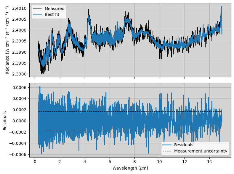
3. Exploring the outputs

3.1. Reading the fitted spectrum

[13]:

Measurement = ans.Files.read_bestfit_hdf5(runname)

[14]:

#Making summary plot
fig,(ax1,ax2) = plt.subplots(2,1,figsize=(8,6),sharex=True)


ax1.plot(Measurement.VCONV,Measurement.MEAS,label='Measured',c='black',linewidth=1)
ax1.plot(Measurement.VCONV,Measurement.SPECMOD,label='Best fit',linewidth=2.)

ax2.plot(Measurement.VCONV,Measurement.SPECMOD-Measurement.MEAS,linewidth=2.,label='Residuals')
ax2.plot(Measurement.VCONV,Measurement.ERRMEAS,c='black',linewidth=1,label='Measurement uncertainty',linestyle='--')
ax2.plot(Measurement.VCONV,-Measurement.ERRMEAS,c='black',linewidth=1,linestyle='--')
ax2.legend()

ax1.grid()
ax2.grid()
ax1.legend()
ax1.set_facecolor('lightgray')
ax2.set_facecolor('lightgray')
ax2.set_xlabel('Wavelength ($\mu$m)')
ax1.set_ylabel('Radiance (W cm$^{-2}$ sr$^{-1}$ (cm$^{-1}$)$^{-1}$)')
ax2.set_ylabel('Residuals')
plt.tight_layout()

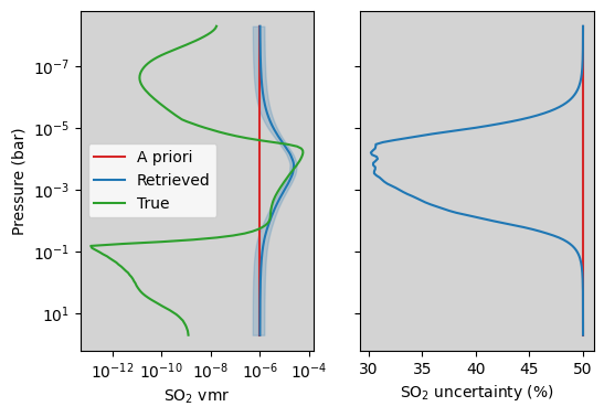
../../_images/examples_retrieval_exoplanet_transit_retrieval_exoplanet_26_0.png

3.2. Reading the retrieved parameters

[15]:

nvar,nxvar,varident,varparam,aprparam,aprerrparam,retparam,reterrparam = ans.Files.read_retparam_hdf5(runname)

[17]:

fig,(ax1,ax2) = plt.subplots(1,2,figsize=(6,4),sharey=True)

ivar = 0

capr = "tab:red"
cret = "tab:blue"
ctrue = "tab:green"

ax1.plot(aprparam[:,ivar],Atmosphere.P/1.0e5,label="A priori",c=capr)
ax1.fill_betweenx(Atmosphere.P/1.0e5,retparam[:,ivar]-reterrparam[:,ivar],retparam[:,ivar]+reterrparam[:,ivar],alpha=0.2,color=cret)
ax1.plot(retparam[:,ivar],Atmosphere.P/1.0e5,label="Retrieved",c=cret)
ax1.plot(Atmosphere.VMR[:,Atmosphere.ID==9],Atmosphere.P/1.0e5,label="True",c=ctrue)
ax1.set_xscale("log")
ax1.set_facecolor("lightgray")
ax1.set_ylabel("Pressure (bar)")
ax1.set_yscale("log")
ax1.set_xlabel("SO$_2$ vmr")
plt.gca().invert_yaxis()

ax2.plot(aprerrparam[:,ivar]/aprparam[:,ivar]*100.,Atmosphere.P/1.0e5,label="A priori",c=capr)
ax2.plot(reterrparam[:,ivar]/retparam[:,ivar]*100.,Atmosphere.P/1.0e5,label="Retrieved",c=cret)
ax2.set_facecolor("lightgray")
ax2.set_xlabel("SO$_2$ uncertainty (%)")

ax1.legend()

[17]:

<matplotlib.legend.Legend at 0x1547fed91250>

../../_images/examples_retrieval_exoplanet_transit_retrieval_exoplanet_29_1.png