Introduction
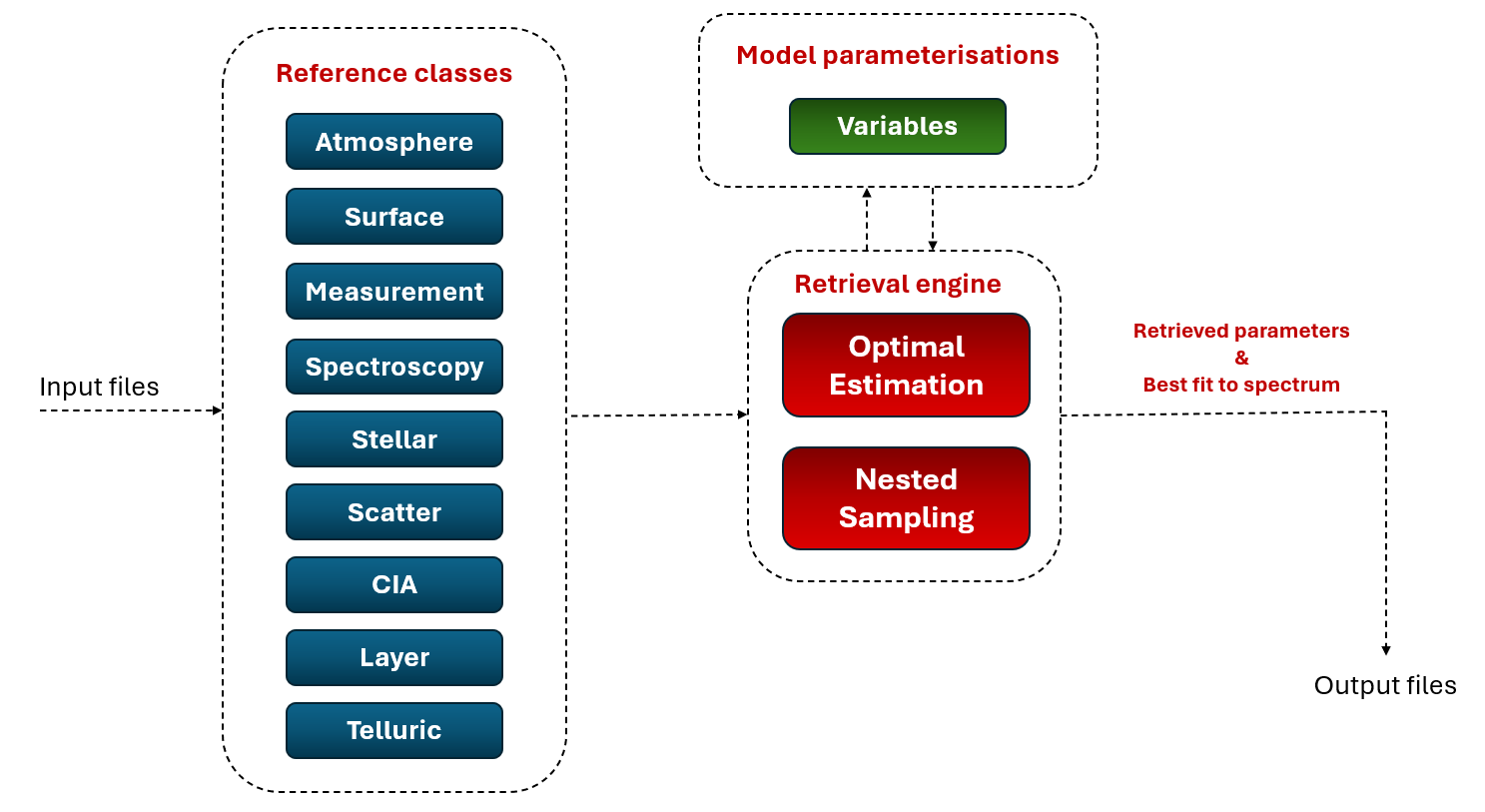
In order to obtain information about the structure and composition of a planetary atmosphere from its electromagnetic spectrum, apart from the radiative transfer model, which relates the atmospheric parameters to the modelled spectrum, we need a retrieval tool to solve the inverse problem, which allows us to estimate what atmospheric parameters provide a best fit between the modelled and measured spectrum. There are several algorithms and techniques that can be applied to solve the inverse problem, each with its own advantages and disadvantages. In archNEMESIS, two different retrieval methodologies can be applied: optimal estimation and nested sampling.
Optimal Estimation
Description of the algorithm
NOTE: A complete description of the implementation of the Optimal Estimation framework in NEMESIS is given in Irwin et al. (2008).
NEMESIS uses the non-linear optimal estimator formalism (Rodgers, 2000), which iteratively minimises the difference between the modelled and measured spectra, subject to a minimum departure from an a priori state of the atmosphere, by minimising the cost function
where \(\mathbf{y}_m\) is the measured spectrum, \(\mathbf{y}_n\) is the synthetic spectrum calculated using the forward model, \(\mathbf{x}_n\) is the state vector, which includes the atmospheric parameters to be retrieved, \(\mathbf{S}_{\epsilon}\) is the measurement covariance matrix, \(\mathbf{x}_a\) is the a priori state vector and \(\mathbf{S}_a\) is the a priori covariance matrix.
For atmospheric sounding in the Earth’s atmosphere, climatology provides good statistics about the a priori state vector and covariance matrix. However, for planetary atmospheres no such statistical record exists, and in that case the diagonal elements of the a priori covariance matrix are set to the square of the estimated errors in the a priori state vector. In the case of retrieving continuous vertical profiles, the values at different altitudes are assumed to be correlated, and the off-diagonal terms of \(\mathbf{S}_a\) are then set to follow
where \(p_i\) represents the pressure at the ith level and \(L_c\) is the correlation length, equivalent to the number of scale heights over which the continuous profile is assumed to be correlated.
The retrieval procedure NEMESIS applies to minimise the cost function is to calculate the state vector in the next iteration as
where \(\mathbf{K}_n\) is the Jacobian matrix at the \(n\)th iteration, which represents the derivatives of spectra at each wavelength with respect to each of the elements in the state vector. However, the convergence of the retrieval using this equation can be unstable due to the great variability of \(\mathbf{K}_n\) over iterations. Instead, NEMESIS uses a scheme based on the Marquardt–Levenberg principal, in which the state vector at the next iteration is modified so that it follows
where \(\lambda\) is initially set to 1. If the spectrum calculated using \(\mathbf{x}'_{n+1}\) reduces the cost function, then \(\mathbf{x}'_{n+1}\) is used as \(\mathbf{x}_n\) in the next iteration, and \(\lambda\) is multiplied by 0.3. In the opposite case, in which \(\mathbf{x}'_{n+1}\) actually increases the cost function, then \(\mathbf{x}_n\) is kept and the value of \(\lambda\) is multiplied by 10. As the code converges, \(\lambda \longrightarrow 0\) and \(\mathbf{x}_n\) tends to the optimal estimate.
The error in the optimal estimate is estimated to be the result of two main contributions. The first contribution is the smoothing error \(\mathbf{S}_s\), which can be regarded as the effect in which the observing system smooths the profile. In such a case, the retrieval can be regarded as an estimate of the smoothed state rather than an estimate of the true state, or what is equivalent, an estimate of the true state, but with an error contribution due to smoothing. This contribution to the retrieved error can be calculated as:
The second contribution to the retrieved uncertainty comes from the propagation of the measurement error to the state vector. The covariance matrix of the retrieval noise can be calculated as
In NEMESIS, the measurement error covariance matrix \(\mathbf{S}_\epsilon\) is assumed diagonal, with each of the diagonal elements corresponding to the measured instrument noise equivalent transmission units. In addition, NEMESIS also allows the introduction of a forward modelling error (e.g., can be used to incorporate uncertainties in the line databases) to the measurement error covariance matrix, to set how well we think we can fit the spectra.
These two main contributions form the total retrieved uncertainty in the state vector, which is given by
Running an optimal estimation retrieval
In order to run the retrieval using the optimal estimation formalism, we need to include some extra parameters with respect to when running a forward model. In particular, the parameters we need to specify are:
The maximum number of iterations (NITER). If NITER is set to -1, then the program will only run a forward model and will calculate the Jacobian matrix, but will not iterate the model parameters to improve the fit between the modelled and measured spectrum. This parameter is either specified in the NEMESIS .inp file or in the archNEMESIS HDF5 file.
The retrieval will stop if a convergence criterion is satisfied - the reduction of the cost function \(\phi\) is lower than a given factor (PHILIMIT). This parameter is either specified in the NEMESIS .inp file or in the archNEMESIS HDF5 file.
The initial model parameters (i.e., \(\mathbf{x}_a\)) and the a priori uncertainties (i.e., \(\mathbf{S}_a\)) are specified in the .apr file. This file is also required when running a forward model, but the information about the uncertainties is only used in retrievals.
Once all the required information has been specified in the input files, we can easily run the retrieval by using the following code.
import archnemesis as ans

legacy_files=True   #(True = standard NEMESIS files ; False = archNEMESIS HDF5 file)
retrieval_method=0  #(0 - optimal estimation ; 1 - nested sampling)
NCores=10           #Number of parallel processes to use for the computations

ans.Retrievals.retrieval_nemesis(runname,legacy_files=legacy_files,retrieval_method=retrieval_method,NCores=NCores)
Once the retrieval has finished, it will write the outputs either to the NEMESIS .mre and .cov files, or to the archNEMESIS HDF5 file. Please read the section about output files to get an insight on how to read the results from optimal estimation retrievals.
Nested Sampling
Introduction
Nested sampling is a Bayesian inference method. The Bayes theorem is mathematically expressed as
\(P(\theta | D) = \dfrac{P(D | \theta) P(\theta))}{P(D)}\),
where \(P(\theta | D)\) is the posterior distribution (i.e, probability of the parameters \(\theta\) given the data \(D\)), \(P(D | \theta)\) is the likelihood (i.e., probability of the data \(D\) given the parameters \(\theta\)), \(P(\theta)\) is the prior distribution (i.e., probability of the parameters \(\theta\) before seeing the data), and \(P(D)\) is the marginal likelihood or the Bayesian evidence,which is a normalising constant ensuring that the posterior distribution integrates to 1.
In standard MCMC sampling methods the evidence is typically ignored and they explore the parameter space to find the posterior distribution. Nested sampling (Skilling 2004) is a Monte Carlo technique aimed at efficient evaluation of the Bayesian evidence, but also produces posterior inferences as a by-product. Therefore, given a set of measured data, nested sampling will explore the parameter space and will provide information about the posterior distribution (i.e., the probability of model parameters given the measured data).
ArchNEMESIS does not include an explicit implementation of the nested sampling algorithm, but uses instead the retrieval engine from pymultinest. This python library relies on the MultiNest nested sampling implementation, which must be compiled before installing pymultinest.
Installing MultiNest
These instructions are paraphrased from the PyMultiNest documentation. For all the details, please see https://johannesbuchner.github.io/PyMultiNest/install.html
PyMultiNest can be installed with:
pip install pymultinest
You should also install Corner for cornerplots:
pip install corner
MultiNest and Cuba must also be installed. First, you must make sure all the prerequisites are present. On Linux, this can be done with:
sudo apt-get install python-{scipy,numpy,matplotlib,progressbar} ipython libblas{3,-dev} liblapack{3,-dev} libatlas{3-base,-dev} cmake build-essential git gfortran
To install and compile Multinest:
git clone https://github.com/JohannesBuchner/MultiNest
cd MultiNest/build
cmake ..
make
To install and compile Cuba:
git clone https://github.com/JohannesBuchner/cuba/
cd cuba
./configure
./makesharedlib.sh
Make sure the packages can find their libraries:
export LD_LIBRARY_PATH=$HOME/Downloads/MultiNest/lib:$HOME/Downloads/cuba/directory/:$LD_LIBRARY_PATH
After this, everything should be ready for nested sampling. Test importing the libraries:
python -c 'import pymultinest'
python -c 'import pycuba'
Installing OpenMPI
PyMultiNest uses MPI for parallelisation, through mpi4py. First, you will have to install a working MPI implementation.
The most reliable way to do this is to build it from source. First, download the source code from the OpenMPI website: https://www.open-mpi.org/software/ompi/v5.0/
Then, install with:
tar xf openmpi-<version>.tar.bz2

cd openmpi-<version>

./configure --prefix=<path> 2>&1 | tee config.out

make all 2>&1 | tee make.out

make install 2>&1 | tee install.out
There are many configuration options, and several different methods of installation. See https://docs.open-mpi.org/en/v5.0.x/installing-open-mpi/quickstart.html for more details.
After this, you can install mpi4py with:
pip install mpi4py
This should install without any errors.
Running a nested sampling retrieval
The initial model parameters (i.e., \(\mathbf{x}_a\)) and the a priori uncertainties are specified in the .apr file. For most parameterisations, the prior distribution of each parameter is specified as a Gaussian in log-parameter space, with a mean equal to the .apr parameter value, and a standard deviation equal to (.apr parameter uncertainty)/(.apr parameter value).
For example, if our .apr file looks like this:
1
Gas ID  Iso ID  Parameterisation ID
1.0  0.1
2.0  0.5
0.1  0.1e-8
Then our first parameter, in log-parameter space, has a mean value of log(1.0) = 0 , and a standard deviation of 0.1/1.0 = 0.1. So our prior distribution is \(N(0,0.1)\).
Similarly, the prior distribution for the second parameter in log-parameter space is \(N(log(2),0.25)\).
The third parameter has an uncertainty less than \(10^{-7}\) times the parameter value, and thus is treated as a constant.
Once we have specified all our prior distributions, we can run the retrieval. Nested sampling requires many more forward model runs than optimal estimation, and so parallelisation is needed. Because PyMultiNest uses OpenMPI, we must launch the retrieval as a new script, outside of the notebook we might be working in. This can be done using python’s inbuilt subprocess module.
import archnemesis as ans

runname = 'runname' # Prefix of .apr, .inp etc.

legacy_files=True   #(True = standard NEMESIS files ; False = archNEMESIS HDF5 file)
retrieval_method=1  #(0 - optimal estimation ; 1 - nested sampling)
NCores=10           #Number of parallel processes to use for the computation

folder_prefix = 'nested_sampling_output/' # Output folder for results - optional

subprocess.run(["mpiexec", "-np", str(NCores), "python", "-c",
                f"import archnemesis as ans; ans.Retrievals.retrieval_nemesis('{runname}', legacy_files={legacy_files}, retrieval_method={retrieval_method}, NCores={NCores}, NS_prefix='{folder_prefix}')"])
Output will proceed. You should see the acceptance rate decrease and the ln(Z) (evidence) value increase towards zero. PyMultiNest writes checkpoint files fairly regularly, so it is possible to pause and unpause a retrieval.
Once the retrieval has finished, a cornerplot (without parameter names) will be produced in the output folder. To load the points in log-parameter space which make up the posterior distribution, you can run:
import numpy as np

output = np.loadtxt(f"{folder_prefix}/post_equal_weights.dat")
posterior_points = output[:,:-1]
loglikelihoods = output[:,-1]

# Printing some statistics:

means = np.exp(np.mean(posterior_points, axis=0))
medians = np.exp(np.median(posterior_points, axis=0))
stdevs = np.std(posterior_points, axis=0)*means

print(f"Means:               {', '.join(f'{x:.2e}' for x in means)}")
print(f"Medians:             {', '.join(f'{x:.2e}' for x in medians)}")
print(f"Standard deviations: {', '.join(f'{x:.2e}' for x in stdevs)}")
This array has N_LIVE_POINTS (normally 400) rows, each corresponding to a single point in the retrieved posterior distribution. The columns correspond to each varying parameter, with the last column corresponding to the evaluated log-likelihood of each point (the log-likelihood is equal to \(-\frac{\chi^2}{2}\)).
You can produce your own cornerplot with, for example:
import corner

parameter_names = ['Parameter 1', 'Parameter 2']

figure = corner.corner(
    posterior_points,
    color="blue",
    bins=50,
    hist_kwargs={'density': True},
    show_titles=True,
    plot_contours=True,
    fill_contours=False,
    contour_colors=["blue"],
    title_fmt=".2e",
    labels = parameter_names,
    smooth = 1.0
    )